Step by step 2D example#
A simple 2D case with symbolic work to illustrate the two-scale library implementation and approach.
Initialization#
The TS library will to be used in parallel in this test. Thus we start by launching an MPI cluster of 2 MPI engines with ipyparallel.
import ipyparallel as ipp
cluster = ipp.Cluster(engines="mpi", n=2)
rc = cluster.start_and_connect_sync()
view=rc[:]
/dolfinx-env/lib/python3.12/site-packages/tqdm/auto.py:21: TqdmWarning: IProgress not found. Please update jupyter and ipywidgets. See https://ipywidgets.readthedocs.io/en/stable/user_install.html
  from .autonotebook import tqdm as notebook_tqdm
Use Twoscale dolfinx implementation
In this context (%%px), we load the components of the TS library and dolfinx
%%px
from dolfinx import mesh
from dolfinx import fem
from dolfinx.fem import petsc
from dolfinx import la


import ufl
import basix

from twoscale import core
from twoscale import linear
from twoscale import util
This test case is very basic and uses, at the coarse scale, a rectangular plate of dimension 2LxL.
%%px
domain= mesh.create_rectangle(MPI.COMM_WORLD,[[0.0, 0.], [2*L, L]],[2,1],ghost_mode=mesh.GhostMode.none)
The numerical application used throughout this document is:
where
\(i_x\) is the imposed displacement along x component to stretch the plate by pulling on right-hand side of the plate.
\(c_x\),\(c_y\) are the imposed displacement along x,y component to block rigid-body modes and clamp left hand side of the plate. Usually set to zero, these arbitrary values are made visible by considering that they can be non-null. Retaining them as explicit variables gives a way to see more clearly their influence in the computation.
\(f\) is the value of the constant imposed volumic load along -x axis
\(E\) is the Young’s modulus
\(\nu\) is the Posson’s ratio
\(L\) is one dimension of the plate
\(\lambda\) and \(\mu\) are the Lamè coefficients
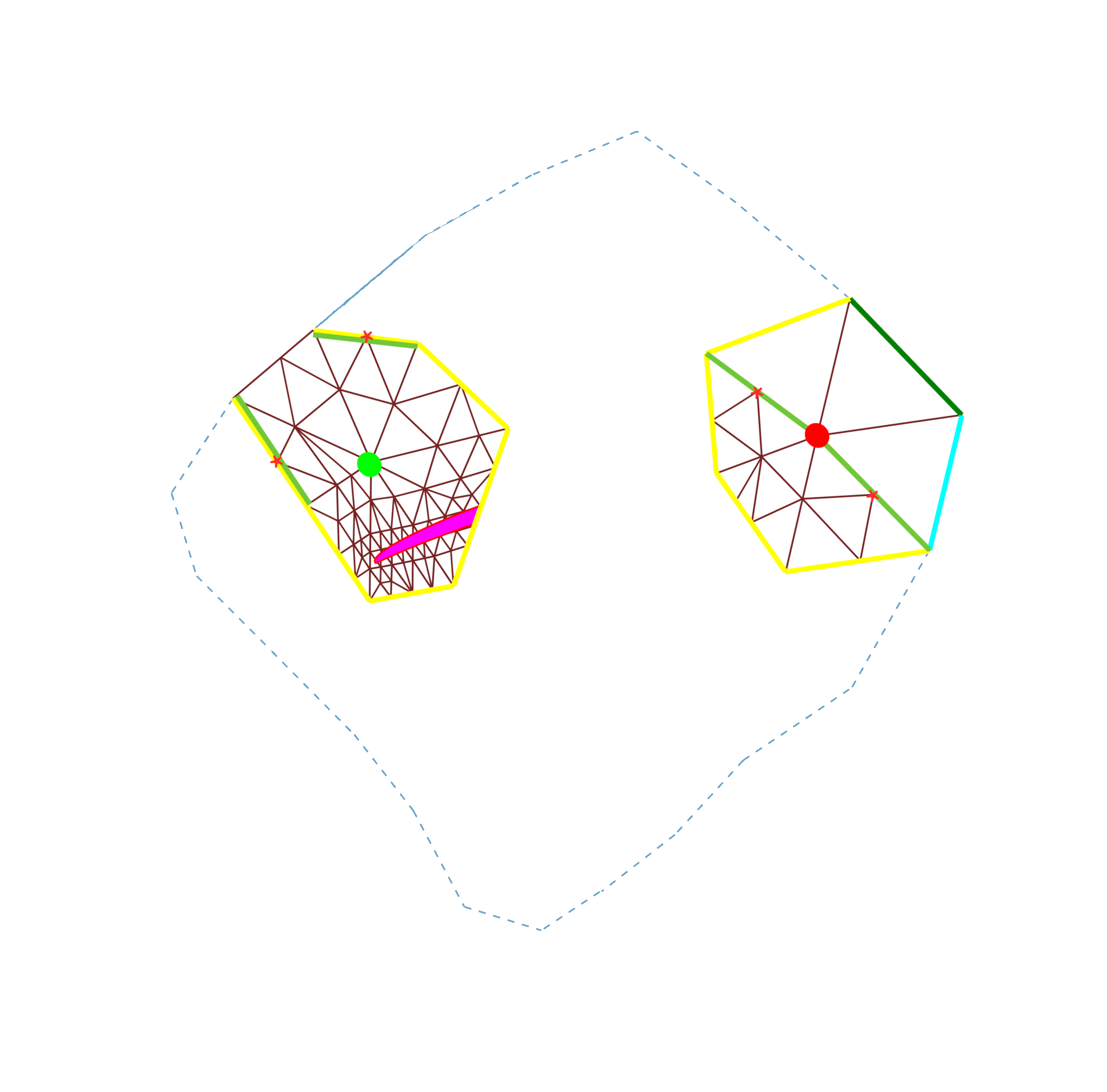
First of all the jump between scale has to be defined. For that the set of enriched nodes and refinement criteria around these nodes needs to be created. In this simple test case all coarse nodes are enriched and all coarse elements are split once. Thus refinement localisation criterion can be anything as TS library always refine at least once all element in the support which is what we are looking for. The following simple function, which returns true for all mesh coordinates, will do the job:
%%px
def crit(coords):
    return coords[0]>-L
And the exact same function can be used for enriched nodes selection (all).
To create a scaleJump object sj that stores all the information required by TS method the only function proposed for now is topDown.
%px sj=core.topDown(domain,crit,crit,1)
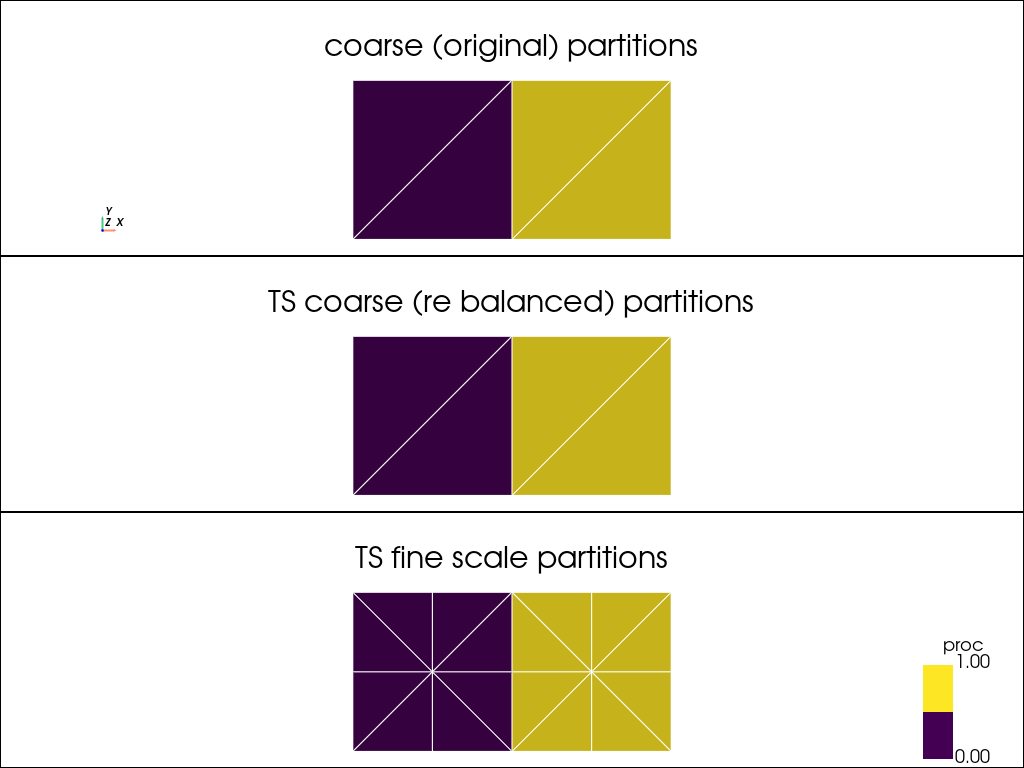
This object sj provides the mesh at both scales (the new coarse mesh is in general a re distributed version of the original coarse mesh according to the set of enriched nodes).
Warning
The mesh argument given to topDown (here domain) should not be used after the call, as it has been transformed and moved inside this function.
Thus, the two meshes at both scales are:
%%px
fdomain=sj.getFineMesh
cdomain=sj.getCoarseMesh
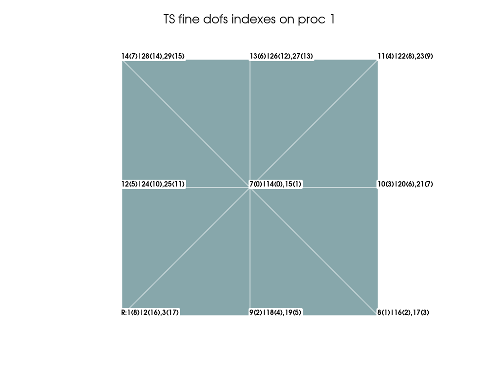
The following shows the discretisation of the 2D problem for the symbolic approach and with TS library
2026-09-23 15:50:42.262 ( 1.725s) [ 7F825B351140]vtkXOpenGLRenderWindow.:1450 WARN| bad X server connection. DISPLAY=
---------------------------------------------------------------------------
ValueError                                Traceback (most recent call last)
Cell In[16], line 22
     18 plt.subplot(0, 0)
     19 plt.add_axes()
     20 plt.add_mesh(grid,show_edges=True,show_scalar_bar=False,scalars=np.array(range(0,4)),edge_color='w')
     21 plt.add_point_labels(xx, labels, point_size=2, font_size=14,shape_color='white')
---> 22 plt.camera_position =cam_pos
     23 plt.add_title("symbolic coarse scale",font_size=12)
     24 idxmgf=domainf.geometry.index_map()
     25 nbdfb=idxmgf.size_local

File /dolfinx-env/lib/python3.12/site-packages/pyvista/core/utilities/misc.py:572, in _NoNewAttrMixin.__setattr__(self, key, value)
    570 if object.__getattribute__(self, '__dict__').get('__frozen_by_class') is type(self):
    571     _NoNewAttrMixin._check_new_attribute(self, key)
--> 572 object.__setattr__(self, key, value)

File /dolfinx-env/lib/python3.12/site-packages/pyvista/plotting/plotter.py:2299, in BasePlotter.camera_position(self, camera_location)
   2297 @camera_position.setter
   2298 def camera_position(self, camera_location: CameraPositionOptions) -> None:
-> 2299     self.renderer.camera_position = camera_location

File /dolfinx-env/lib/python3.12/site-packages/pyvista/core/utilities/misc.py:572, in _NoNewAttrMixin.__setattr__(self, key, value)
    570 if object.__getattribute__(self, '__dict__').get('__frozen_by_class') is type(self):
    571     _NoNewAttrMixin._check_new_attribute(self, key)
--> 572 object.__setattr__(self, key, value)

File /dolfinx-env/lib/python3.12/site-packages/pyvista/plotting/renderer.py:584, in Renderer.camera_position(self, camera_location)
    582     self.camera.position = scale_point(self.camera, camera_location[0], invert=False)
    583     self.camera.focal_point = scale_point(self.camera, camera_location[1], invert=False)
--> 584     self.camera.up = camera_location[2]
    586 # reset clipping range
    587 self.reset_camera_clipping_range()

File /dolfinx-env/lib/python3.12/site-packages/pyvista/core/utilities/misc.py:572, in _NoNewAttrMixin.__setattr__(self, key, value)
    570 if object.__getattribute__(self, '__dict__').get('__frozen_by_class') is type(self):
    571     _NoNewAttrMixin._check_new_attribute(self, key)
--> 572 object.__setattr__(self, key, value)

File /dolfinx-env/lib/python3.12/site-packages/pyvista/plotting/camera.py:510, in Camera.up(self, vector)
    508 if np.allclose(vector, 0.0):
    509     msg = 'Camera up vector cannot be zero.'
--> 510     raise ValueError(msg)
    511 self.SetViewUp(vector)
    512 self.is_set = True

ValueError: Camera up vector cannot be zero.
[output:0]
[output:1]
[output:0]
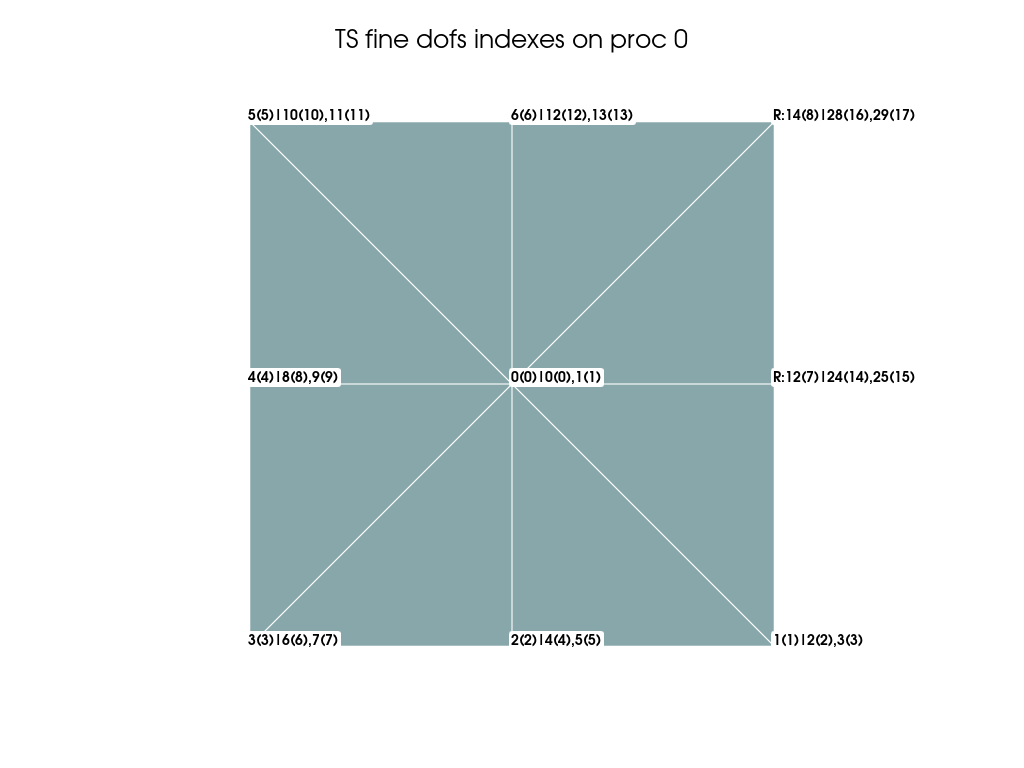
Fine scale level#
The fine scale system#
Fine-scale triangles have edge sizes of \(\frac{L}{2}\) and \(\frac{L.\sqrt{2}}{2}\) and the elementary matrix associated with one fine triangle is given by \(ke = t_e.area_e.C^t.M.C\) with:
\(t_e\) the thickness taken as 1.
\(area_e\) the area, which is \(\frac{1}{2}.\frac{L}{2}.\frac{L}{2}=\frac{L^2}{8}\)
Using the lamè coefficients \(\lambda\), \(\mu\) the isotropic plan strain stiffness matrix \(M\) is:
And C for a triangle of category 0 is
and for a triangle of category 1 C is
and for a triangle of category 2 C is
and for triangle of category 3 C is
Thus, the elementary matrices for triangles of categories 0, 1, 2 and 3 are:
With TS library/FEniCSx elementary matrices are defined through the formulation:
%%px
#space
space = fem.functionspace(fdomain, fdomain.ufl_domain().ufl_coordinate_element())
#lamè
mu=fem.Constant(fdomain,E / (2.0 * (1.0 + nu)))
lmbda = fem.Constant(fdomain,E * nu / ((1.0 + nu) * (1.0 - 2.0 * nu)))
#trial/test
u = ufl.TrialFunction(space)
v = ufl.TestFunction(space)
# strain
def eps(v):
    return 0.5*(ufl.grad(v) + ufl.grad(v).T)
# stress
def sigma(strain):
    return 2.0*mu*strain + lmbda*ufl.tr(strain)*ufl.Identity(2)
#  bilinear formulation
a=ufl.inner(sigma(eps(u)), eps(v)) * ufl.dx
In symolic treatment standard system matrix A at fine scale is than given by assembling \(Ke_0\), \(Ke_1\), \(Ke_2\) and \(Ke_3\),for each element of each category:
All symbolic numerical conterpart are identified with a trealing \(N\) in their name and are optionaly visible using drop down widget.
The elementary load vector associated to one fine triangle is given by \(Fe = t_e.\int N^t.fn.dV\) with \(fn=[-f,0]\) considering only constant volumic load along -x component. Integration gives for all element category:
Standard system rhs B is than by assemble \(Fe\) for each element :
Equivalently, with the TS library/FEniCSx, the volumic load is set by imposing \([-f,0]\) as a constant field
%%px
#constant
fv=fem.Constant(fdomain,[-f,0.])
#linear formulation
b=ufl.dot(fv,v)*ufl.dx
Dirichlet operator used in this work follows PETSc/FEniCSx logic:
Dirichlet dofs rows and columns of the system matrix are nullified by application of a \(D\) operator (identity matrix with 0 on Dirichlet dofs diagonal position)
The Dirichlet dofs diagonal position are set to 1 by adding a \(U=\mathbb{I}-D\) matrix to filtered \(A\) matrix (i.e. \(D^t.AD\))
The Dirichlet dofs values are set in a vector \(X_D\)
The rhs \(B\) is filtered by \(D\)
\(X_D\) is added to rhs
The coupling terms related to imposed Dirichlet values (\(D^t.A.X_D\)) is substracted to rhs
For this test case the following Dirichlet boundary conditions values are set for symbolic problem:
dofs (0,1,20) are fixed repectively with \(c_x\), \(c_y\) and \(c_x\) arbitrary values.
dofs (8,18,28) are fixed with \(i_x\) (traction)
Dirichlet boundary condition with TS library/FEniCSx resume to identify dofs and associate values to them:
%%px
bc_nodes_1=mesh.locate_entities(fdomain, 0, lambda x: np.isclose(x[0], 0.))
bc_dofs_1=fem.locate_dofs_topological(space.sub(0),0,bc_nodes_1)
bc1=fem.dirichletbc(np.array(cx),bc_dofs_1,space.sub(0))
bc_nodes_2=mesh.locate_entities(fdomain, 0, lambda x: np.isclose(x[0], 2*L))
bc_dofs_2=fem.locate_dofs_topological(space.sub(0),0,bc_nodes_2)
bc2=fem.dirichletbc(np.array(ix),bc_dofs_2,space.sub(0))
bc_nodes_3=mesh.locate_entities(fdomain, 0, lambda x: np.logical_and(np.isclose(x[0], 0.),np.isclose(x[1], 0.)))
bc_dofs_3=fem.locate_dofs_topological(space.sub(1),0,bc_nodes_3)
bc3=fem.dirichletbc(np.array(cy),bc_dofs_3,space.sub(1))
bcs=[bc1,bc2,bc3]
In symbolic approach, has mentionned above, applying Dirichlet BC resume to:
\(AD=D^t.A.D+U\)
\(BD=-D^t.A.X_D+X_D+D^t.B\)
Has \(D^t=D\) it simplify to:
\(AD=D.A.D+U\)
\(BD=-D.A.X_D+X_D+D.B\)
Sytem matrix after Dirichlet BC is thus:
For TS library/FEniCSx the linear, bilinear ufl formulation and the Dirichlet BC can now be used to create \(A\),\(B\),\(AD\),\(BD\) matrices.
To simplifify implementation the use of createFineScaleSytems will hide all the creation and assembly aspect of those matrices.
%%px
[A,AD,B,BD]=util.createFineScaleSytems(a,b,bcs=bcs)
Solution at fine scale#
\(S_F=AD^{-1}.BD\)
Semi numerical application
With TS library/FEniCSx \(AD\), \(BD\) system is solve with PETSc:
%%px
petsc_options={"ksp_type":"preonly","pc_type":"lu","pc_factor_mat_solver_type":"mumps"}
solverf = petsc4py.PETSc.KSP().create(fdomain.comm)
solverf.setOperators(AD)
opts = petsc4py.PETSc.Options()
for k, v in petsc_options.items():
    opts[k] = v
solverf.setFromOptions()
sf=fem.Function(space)
x_sf = sf.x.petsc_vec
solverf.solve(BD, x_sf)
sf.x.scatter_forward()
A sequential FEniCSx implementation (in drop down bellow) provides a way to do direct comparison with symbolic computation:
Numerical field difference between symbolic and sequential FEniCSx resolution
 x                     y
[[ 1.90819582e-17 -1.21430643e-17]
 [ 0.00000000e+00 -2.25514052e-17]
 [ 0.00000000e+00 -1.12757026e-17]
 [ 8.67361738e-18 -1.73472348e-17]
 [ 0.00000000e+00  0.00000000e+00]
 [ 1.38777878e-17 -7.80625564e-18]
 [ 8.23993651e-18 -1.04083409e-17]
 [ 1.56125113e-17 -9.54097912e-18]
 [ 1.38777878e-17 -1.38777878e-17]
 [ 1.38777878e-17 -9.54097912e-18]
 [ 1.38777878e-17  0.00000000e+00]
 [ 6.93889390e-18 -1.38777878e-17]
 [ 0.00000000e+00 -6.93889390e-18]
 [ 0.00000000e+00 -3.46944695e-17]
 [ 0.00000000e+00 -1.99493200e-17]]
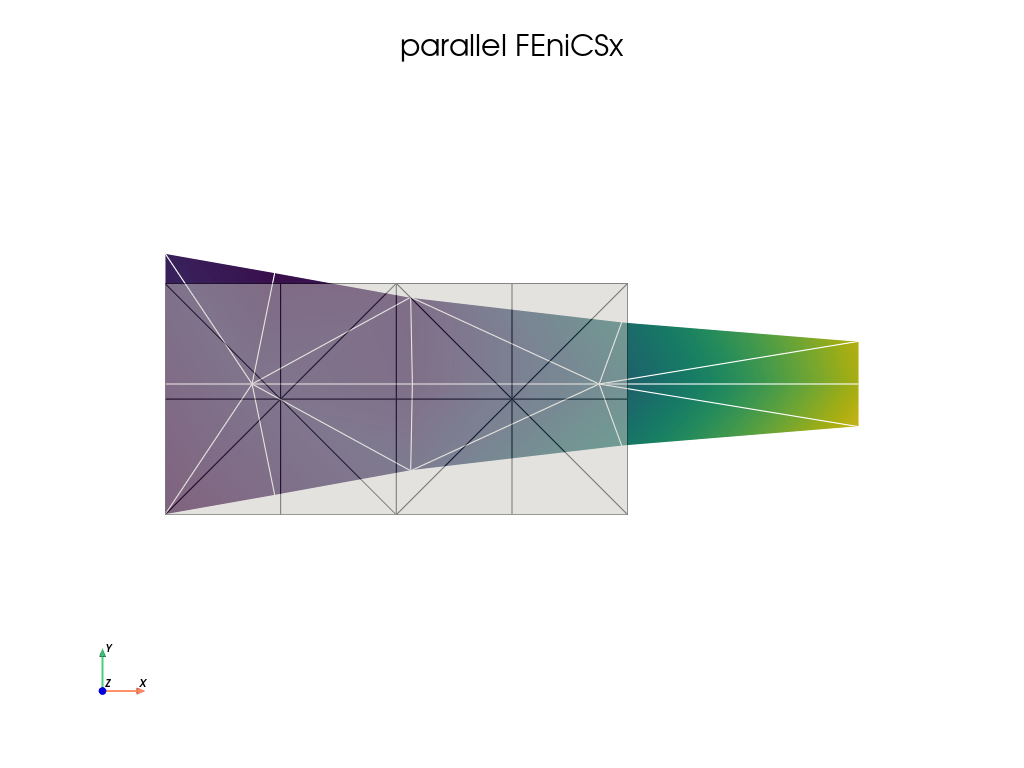
visualisation with scale factor
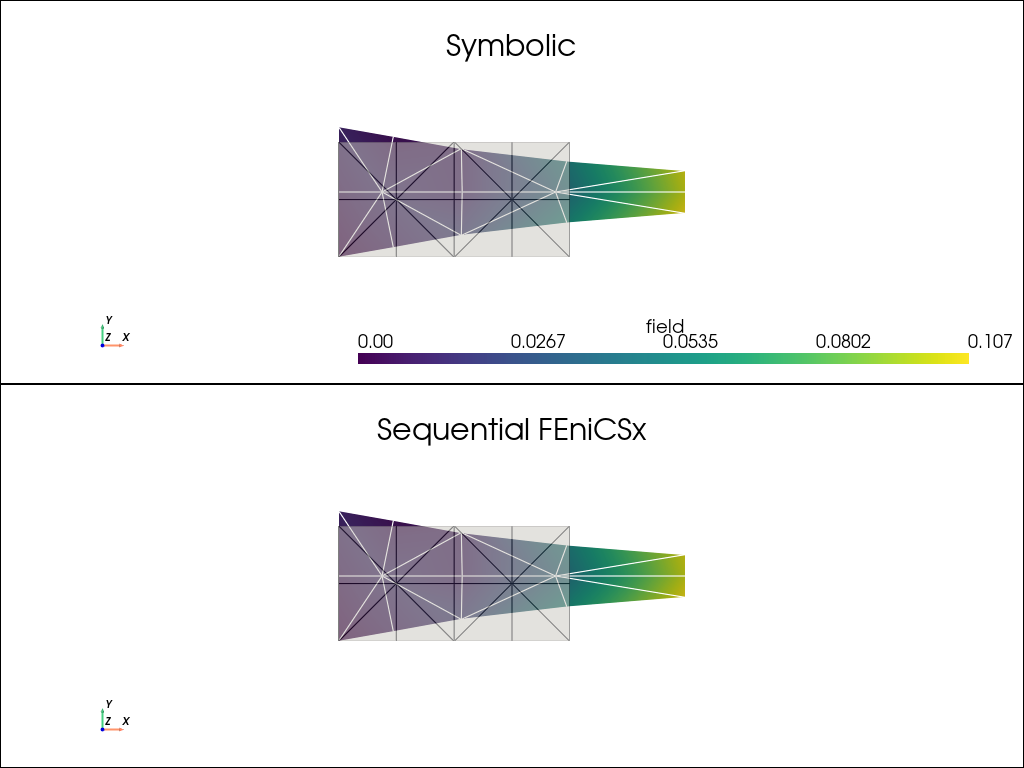
[output:0]
Coarse scale level#
Coarse non enriched system#
Compare to fine scale we have only two element categories.
The elementary stifness matrix are the same as fine scale ones.
The elementary load are the same as fine scale ones muliplied by 4
This gives the folowing matrices:
Solution at coarse scale without enrichment#
Semi numerical application
Numerical application
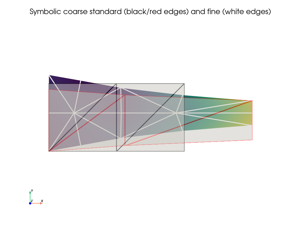
Equivalent solution with TS library/FEniCSx#
In the following hidden cells, a FEniCSx definition of the coarse non enriched problem is given:
It’s resolution is given by:
%%px
problem_cs = petsc.LinearProblem(a_cs, b_cs,bcs=bc_cs,petsc_options=petsc_options,petsc_options_prefix="cs_")
disp_cs = problem_cs.solve()
[stdout:0] [ 0.          0.          0.0125     -0.01666667  0.         -0.00833333
  0.0125      0.00833333]
[stdout:1] [ 0.0125      0.00833333  0.1         0.01666667  0.1        -0.025
  0.0125     -0.01666667]
Two scales level#
Coarse enriched field#
At coarse scale the field must be enriched to be able to promote fine scale results at coarse scale. In this test case, as all coarse dofs are enriched, the enriched space is equivalent to the standard coarse dof space.
For the symbolic application, we will consider that standard DOFs comme first (0,…11) and enriched dof after (12,…23) with the same ordering (see figure in sections).
Library has been compiled for 'nested' strategy
Thus all mention of 'monolithic' can be ignored in remaining part of this document
For TS library/FEniCSx we will consider a mixed space of two simple Lagrange order 1 spaces grabed from mesh definition for monolithic strategy:
%%px

el_mixed = basix.ufl.mixed_element([cdomain.ufl_domain().ufl_coordinate_element(), cdomain.ufl_domain().ufl_coordinate_element()])
coarse_enriched_space = fem.functionspace(cdomain, el_mixed)
[output:1]
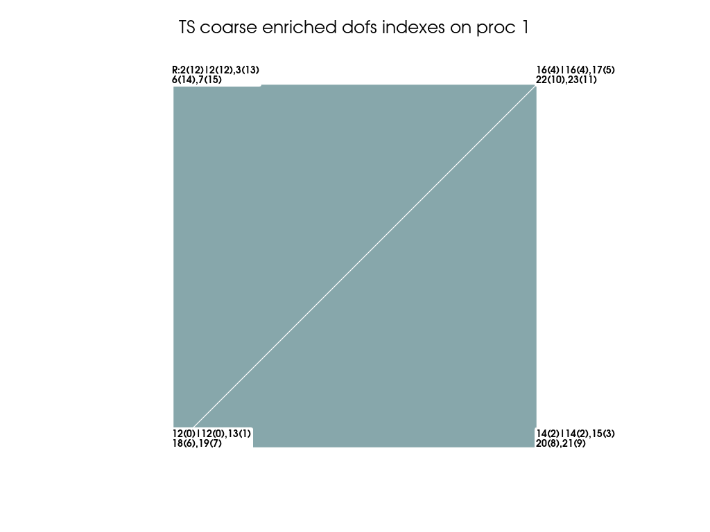
[output:0]
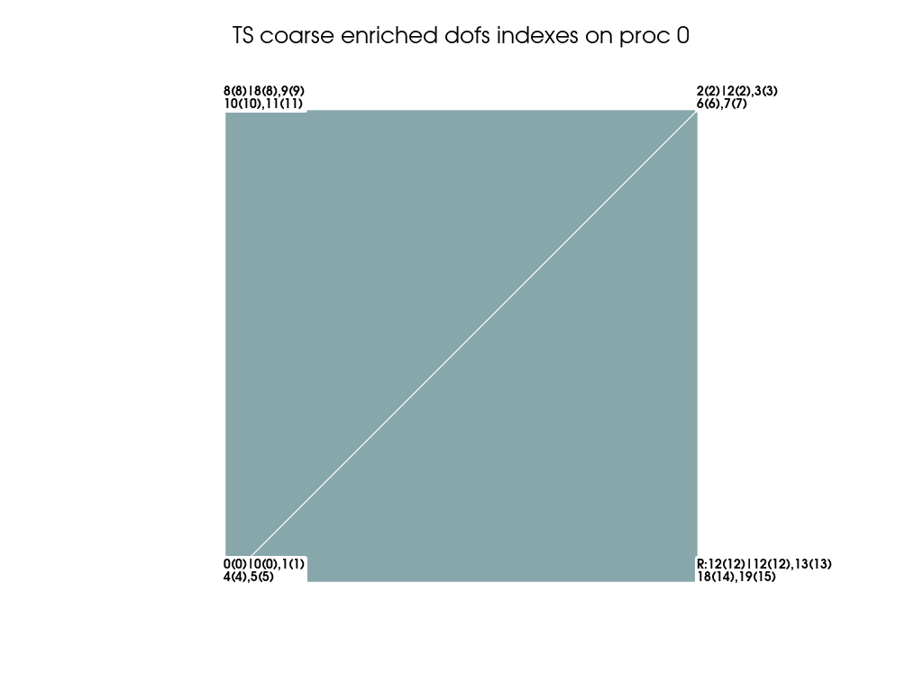
And the enriched field is thus:
%%px
Sce=fem.Function(coarse_enriched_space,name='field_coarse_enriched')
if not nested_strategy:
    coarse_field=Sce
    coarse_space=coarse_enriched_space
For TS library/FEniCSx using nested strategy we will consider two separate simple Lagrange order-1 spaces grabbed from the mesh definition. But only one will be given to the library: the standard coarse space. The other one (the enriched space) is constructed internally by the library and may span only on a submesh (If not all nodes are enriched which is not the case in this test case). A simple way to implement this is to use directly the field obtained in the coarse computation:
%%px
if nested_strategy:
    coarse_field=disp_cs
    coarse_space=space_cs
Boundary conditions at both scale#
In all approaches the Dirichlet boundary conditions are imposed in the same way at both scale. At fine scale it has already been taken into account with the creation of \(AD\),\(BD\) from \(A\),\(B\) with createFineScaleSytems function. At coarse scale the TS library expects with the monolithic approach a unique DirichletBC object to impose BC. The detailled procedure is given in “exemple of dirichlet boundary condition setting for the coarse enriched problem “ and adapted to the current test case where only standard dofs are imposed. Thus to selectively impose boundary condition sub space are needed with monolithic approach:
%%px

std_=coarse_enriched_space.sub(0)
std, std_to_mix=std_.collapse()
enr_=coarse_enriched_space.sub(1)
enr, enr_to_mix=enr_.collapse()
Like at fine scale, nodes with imposed BS need to be identified:
%%px
bc_cnodes_1=mesh.locate_entities(cdomain, 0, lambda x: np.isclose(x[0], 0.))
bc_cnodes_2=mesh.locate_entities(cdomain, 0, lambda x: np.isclose(x[0], 2*L))
bc_cnodes_3=mesh.locate_entities(cdomain, 0, lambda x: np.logical_and(np.isclose(x[0], 0.),np.isclose(x[1], 0.)))
Dofs are then selectively identified from these nodes and subspace. Unique boundary condition object is then created (again see here for more detail) :
%%px
bc_cdofs_1=fem.locate_dofs_topological(std.sub(0),0,bc_cnodes_1)
bc_cdofs_2=fem.locate_dofs_topological(std.sub(0),0,bc_cnodes_2)
bc_cdofs_3=fem.locate_dofs_topological(std.sub(1),0,bc_cnodes_3)
#imposed values will be stored in a field
all_BC_values=fem.Function(coarse_enriched_space)
#by default this fiel is with null values
#only dof related to bc_cnodes_2 need to be set to ix
#For that indirection is created
std_to_mix_np=np.asarray(std_to_mix[0])
bc_cdofsce_2=std_to_mix_np[bc_cdofs_2]
all_BC_values.x.array[bc_cdofsce_2]=ix
# the unique bc object is then
all_BC_dof=np.concat((std_to_mix_np[bc_cdofs_1],bc_cdofsce_2,std_to_mix_np[bc_cdofs_3]))
all_BC_dof.sort()
if not nested_strategy:
    bcc=[fem.dirichletbc(all_BC_values,all_BC_dof)]
With nested strategy bcc is simply the boundary condition created at coarse scale level
%%px
if  nested_strategy:
    bcc=bc_cs
Fine to coarse operator: standard part#
Operator \(PS\) (S for standard part)
rows (fine): dofs (0,..29)
columns (coarse): std dof (0,…11) first enriched (12,…23) second
only standard part expressed thus column from 12 to 23 are null. By hand for symbolic computation it is:
Apply this operator to A we should normaly obtain Acs:
Which is the case.
With the TS library \(PS\) is created when coarseManager object is created with the use of the function generateCoarseManager:
%%px
cm =core.generateCoarseManager(sj,space,coarse_space,None,bcc)
TwoScale loop initialization#
To initialize TwoScale loop in general we use the solution Scs and project it at fine scale with PS to get a starting approximation \(Sts_0=PS.[Scs, 0]^t\):
which is naturally not equal to \(S_F\) when \(f\neq 0\).
With TS library the FEniCSx computation at coarse scale is used by projectStdCoarse method but results must be stored in enriched field with monolithic strategy.
%%px
if not nested_strategy:
    coarse_field.x.array[std_to_mix_np]=disp_ce.x.array
And finaly the projection is done using projectStdCoarse method of cm instance
%%px
Sts0=fem.Function(space)
cm.projectStdCoarse(coarse_field,Sts0)
#Sts0.x.scatter_reverse(la.InsertMode.add)
Sts0.x.petsc_vec.view()
Compare to symbolic computation the TS library provides the same projection (see below).
Patch resolution#
\(Sts_0\) provides information to impose BC to patches
Here the sympbolic resolution of the first patch(in drop down).
Has can be seen, it is to complex to use symbolic expression. We are going to switch to symbolic variables for patch solution and thus for enrichement function but for some computation we will use the solution coresponding to numerical application:
Symbolic dofs used for patch computation:
Patch problem for enriched dof (12,13): free/BC [0, 1, 2, 3, 10, 11, 12, 13, 20, 21, 22, 23] TS BC [4, 5, 14, 15, 24, 25] shift idx [0, 1]
Patch problem for enriched dof (14,15): free/BC [2, 3, 4, 5, 6, 7, 8, 9, 14, 15, 16, 17, 18, 19, 26, 27, 28, 29] TS BC [0, 1, 12, 13, 24, 25] shift idx [2, 3]
Patch problem for enriched dof (16,17): free/BC [6, 7, 8, 9, 18, 19] TS BC [4, 5, 16, 17, 28, 29] shift idx [2, 3]
Patch problem for enriched dof (18,19): free/BC [10, 11, 20, 21, 22, 23] TS BC [0, 1, 12, 13, 24, 25] shift idx [2, 3]
Patch problem for enriched dof (20,21): free/BC [0, 1, 2, 3, 10, 11, 12, 13, 14, 15, 20, 21, 22, 23, 24, 25, 26, 27] TS BC [4, 5, 16, 17, 28, 29] shift idx [14, 15]
Patch problem for enriched dof (22,23): free/BC [6, 7, 8, 9, 16, 17, 18, 19, 26, 27, 28, 29] TS BC [4, 5, 14, 15, 24, 25] shift idx [10, 11]
With TS library/FEniCSx patches are managed by an instance of patchManager class create by generatePatchManager:
%%px
pm =core.generatePatchManager(sj,space)
This instance is responsible of the creation of the patches problem extracted from \(AD\),\(BD\) matrices. Note that patch problem generation expect that Dirichlet boundary condition are already imposed to the fine scale matrices.
%%px
pm.generateProblems(AD,BD)
As soon as patches problem are created they can be solved imposinging current TS approximation (i.e.\(Sts_0\)):
%%px
pm.solveProblems(Sts0)
At this stage patch solutions from TS library can be checked. Normally every symbolic solution can be found in one computing sequence that groupe resolution of 1 or more patches. In this example we have 4/5 sequences that computes 6 patches:
Symbolic solution of patch 0 is identified in TS library sequence 2
Symbolic solution of patch 1 is identified in TS library sequence 1
Symbolic solution of patch 2 is identified in TS library sequence 2
Symbolic solution of patch 3 is identified in TS library sequence 3
Symbolic solution of patch 4 is identified in TS library sequence 0
Symbolic solution of patch 5 is identified in TS library sequence 3
Fine to coarse operator in the general case#
We use the following for the symbolic computation
\(\theta_i\): enriched values at shift dof (so we can easily turn them to zero when using shift enrichment function)
\(\alpha_i^j\): a priori non null enriched function values for pathch related to DOF (i) and for fine DOF (j)
and set \(PG\) (G for general case) using \(PS\) and those variables:
TS approch (I) in general case#
Applying \(PG\) to \(A\) matrix lead to the following expression of the coarse enriched matrix:
it’s rank is to difficult to obtain symbolicaly so we try to get information by passing by numerical equivalent:
With sympy rank method it is not rank deficient ?
Translating symbolic numerical values into numpy float, it is then possible to use matrix_rank function of numpy. We obtain :
As the standard part naturaly exibite 3 rigides body modes and as deficiancy is of 3 we can conclude that the only rigide body modes to block are the one coresponding to standard part. Thus in our case we use Dirichlet boundary condition for that with the natural choice to impose the same condiditons at both scale.
Thus imposing Dirichlet at coarse scale lead to add equations of the from:
\(x_k+\theta_i\times x_i=c\)
with \((k,i)\in\{(0,12),(1,13),(4,16),(6,18),(10,22)\}\)
Which coresponds to the use of a prolongation matrix \(R\) and fixed value \(RF\) if we eliminate (k) standard dofs:
The coarse enriched matrix is in its general forme:
Again with sympy, rank looks correct numericaly. But we check with numpy to be sure:
Thus explicite enriched dof elimination does not look mandatory and for now we do note introduce any.
The rank is correct and we can now create the system.
So the matrix \(AG_C\) and \(BG_C\) are given by applying \(PG\) and \(R\),\(RF\):
Reduced solution \(SG_r\) at coarse scale is:
And the full solution \(SG\) at the coarse scale is:
Fine to coarse operator in the shift case#
If the enriched function is a shifted version of the patch solutions all \(\theta_i\) are null by construction which lead to the following particular operator \(P\) :
TS approach (I) in shift case#
Applying \(P\) to \(A\) matrix lead to the following expression of the coarse enriched matrix:
which is again full rank numerically with sympy. With numpy:
which is again full rank-deficient with 3 modes.
Again use of similar Dirichlet boundary condition at both scale leads to imposing, at the coarse scale, the following equations:
\(x_k=c\)
with \(k \in\{0,1,4,6,10\}\)
that can be treated by simple Dirichlet boundary conditions operator without restriction operator as is done by FEniCSx/PETSc.
For the enriched sub bloc, like in the general case no extra Dirichlet boundary condition are imposed.
The Dirichlet operator are then:
Applying those operator to \(P^t.A.P\) gives the final \(A_C\) matrix:
Which has a correct rank both with sympy and numpy.
Applying \(P\) operator and Dirichlet operator gives the following rhs \(B_C\):
Solution \(S_C\) at coarse scale is then:
Note that \(Sc\) an \(SG_C\) are note the same numericaly as enrichment function are different.
With shift enrichment standard dofs represent the physical displacement which is not the case in general case. Nevertheless enriched dofs are the same. Why ? Euhhh … Erichement functions have the same shape and are just a translation of one another. So we can imagine that only the shape impose the solution of enriched dofs ….
Any way those two solutions projected with their operators gives the same approximates fine scale field:
Compare inital and new approximation with fine solution give:
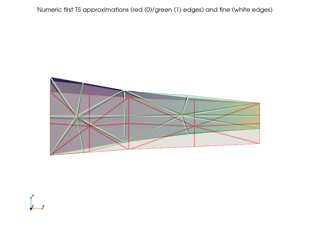
The residual norm of those approximation are:
Doing more up-down symbolic Two Scale resolution gives:
Text(0, 0.5, '$norm(AD.Sts_i-BD)/norm(BD)$')
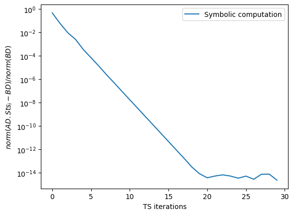
Comparatively the direct fine scale resolution gives with direct numeric(simpy) resolution:
TS approach (II) in shift case#
From an implementation point of view it would be efficient if the TwoScale solver use \(AD\) and \(BD\) directly avoiding creation/storing \(A\),\(B\).
Thus on this specific case we check here that this approch does not work.
First apply \(P\) (or \(PG\), but here we will check only the shift case):
\(AP_C^2=P^t.AD.P\)
\(BP_C^2=P^t.BD\)
Matrix is numericaly full rank with clearly wrong terms comming from the fact that some row/columns in \(AD\) has been replace by identity diagonal sub matrix:
Applying bluntely Dirichlet operator
\(A_C^2=DC^t.AP_C^2.DC+IDC\)
\(B_C^2=XD_C+DC^t.BP_C^2-DC^t.AP_C^2.XD_C\)
gives:
Compaire to \(A_C\), \(A_C^2\) gives almost the same matrix because the wrong terms are eliminated by \(DC\) operator in standard part but unforunately not in enriched and coupled parts as already analysys in theoric section.
For \(B_C^2\) it is the same, terms are not the same.
TS approach (III)#
As mentioned in theoric section
this approach only proposed in the shift case, use:
\(Q=P.D_C\)
\(W_S=P_S.X_{DC}\)
\(Z_S=A.W_S\)
under the condition that \(X_{DCE}=0\) which is the case here.
The assocated system is then
Compare to approch (I) we have
So the solution of this system will be the same as the one of the approach (I)
It is this approach that as been retained for the implementation of the TS library. Thus the coarse system is generated by the cm instance as follows. Before looping, \(Z_C\) and the standard constant part of \(A_C^3\) and \(B_C^3\) are computed out of \(A\),\(B\):
%%px
cm.setStdCoarse(A,B)
To continue we must create the enriched function
%px enriched_shift=core.generateEnrichedShiftFunction(sf)
And then use the last computed solution of the patches to set the enriched part of the \(Q\) operator:
%px cm.updateEnrichedOperator(pm,enriched_shift)
At this stage \(Q\) is fully created and \(A_C^3\),\(B_C^3\) can be finalised by computing all missing blocks from \(A\),\(B\) and \(Q\)
%%px
#cm.resetCoarseToStd()
cm.updateEnrichCoarse(A,B)
The system \(A_C^3\),\(B_C^3\) is now created and can be solved. The library updates the TS approximation in the same call.
%%px
Sts1=fem.Function(space)

cm.solve(Sts1)
The residual norm of \(AD\),\(BD\) system is given for the first two approximation by:
%%px
nb=BD.norm()
Sts0p=Sts0.x.petsc_vec
Sts1p=Sts1.x.petsc_vec
#nb=linear.residual(AD,BD,Sts0p,1)

normsts0=linear.residual(AD,BD,Sts0p,nb)
normsts1=linear.residual(AD,BD,Sts1p,nb)
[output:0]
' norm(AD.Sts_0-BD)/norm(BD)=0.4617363128077323'
[output:0]
' norm(AD.Sts_1-BD)/norm(BD)=0.058547577746052605'
Then loop on level gives
%%px
convTS_curv=[normsts0,normsts1]
Stsi=fem.Function(space)
Stsi.x.array[:]=Sts1.x.array
for i in range(2,30):
    pm.solveProblems(Stsi)
    cm.resetCoarseToStd()
    cm.updateEnrichedOperator(pm,enriched_shift)
    cm.updateEnrichCoarse(A,B)
    cm.solve(Stsi)
    normstsiN=linear.residual(AD,BD,Stsi.x.petsc_vec,nb)
    if i<10 :
        if MPI.COMM_WORLD.rank<1:
            display(f' norm(AD.Sts_{i}-BD)/norm(BD)={normstsiN}')
    convTS_curv.append(normstsiN)
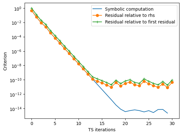
mplt.plot(conv_curv,label='Symbolic computation')
mplt.plot(view['convTS_curv'][0],label='Library computation')
mplt.legend()
mplt.yscale('log')
mplt.xlabel('TS iterations')
mplt.ylabel('$norm(AD.Sts_i-BD)/norm(BD)$')
Text(0, 0.5, '$norm(AD.Sts_i-BD)/norm(BD)$')
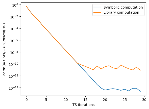
With TS library/FEniCSx all the steps above are grouped in linearBasicLoop function that use two criterions to stop the loop:
a maximum number of iterations
a threshold under which relative system residual is considered as small as needed. Relativeness is either against rhs norm (hrb) or first residual value (hrr).
%%px
[dispf, r,nm, it,hrb,hrr]=linear.linearBasicLoop(sj,space,A,AD,B,BD,enriched_shift,coarse_field,None,bcc,30,1e-13)
Text(0, 0.5, 'Criterion')