Plug the method in FEniCSx : standard workflow with FEniCSx 0.9#
Bottom Up#
\(A_f\),\(b_f\) are assembled and structured by FEniCSx with use of a fine scale space with or without MPC.
For each patch \(p\), \(A_p\) is extracted once from \(A_f\) and factorized once with Mumps.
For each patch \(p\), \(\bar b_p\) is extracted once from \(b_f\) and \(b_p\) is recomputed by adding the current patch Dirichlet BC contribution to \(\bar b_p\).
Monolithic approach#
At coarse level a FEniCSx mixed space is used to represent standard and enriched dof thus \(A_{ce}^i\) is a monolithic matrix
Same for \(b_{ce}^i\) being a vector with standard and enriched DOFs.
The \(P_S\) operator is computed once with FEniCSx providing interpolation coefficients by use of coarse element FF.
\(P_E(x_p^i)\) is compute at each TS iteration from \(P_S\) and \(x_p^i\).
Both operators have the same size as \(A_{ce}^i\)
PETSC multiplication from \(A_f\),\(b_f\) with \(P_S\) and \(P_E(x_p^i)\) provides \(A_{ce}^i\) and \(b_{ce}^i\) in a “block” manner: \(P_S^t.A_f.P_S\) for example, correspond to the standard x standard block of \(A_{ce}^i\) even though it is spread in \(A_{ce}^i\). Unfortunately PETSC provides only matrix matrix multiplication but does not add the result to a resulting matrix. Thus adding \(P_E^t.A_f.P_E\) to \(A_{ce}^i\) requires two steps:
storing \(P_E^t.A_f.P_E\) in a temporary matrix \(T\)
adding \(T\) to \(A_{ce}^i\)
This leads to storing part of \(A_{ce}^i\) twice. Because for efficiency \(T\) must be stored to keep symbolic multiplication analysis which costs a lot.
Coarse enriched system is solved with a Mumps.
Attention
Due to this high memory and computational cost the Nested approach was introduced and may become the reference approach.
Note
But one alternative has not been studied:
merging \(P_S\) and \(P_E\) into a \(P^i\) operator update at each iteration
obtaining \(A_{ce}^i\) and \(b_{ce}^i\) with a simple matrix matrix multiplication (\(P^{it}.A_f.P^i\))
A priori, this does not look efficient has the standard x standard bloc is recomputed at every iteration, even though it is constant. And both coupling blocks are computed even if one is the transpose of the other. But the symbolic multiplication analysis being constant, it can be stored in \(A_{ce}^i\) and reused at each iteration. It may offer good performance and avoid any extra memory consumption.
Nested approach#
At coarse level two FEniCSx spaces are used to represent standard and enriched DOFs thus \(A_{ce}^i\) is a PETSC nested matrix
For now nested features of FEniCSx are not used as the blocks are not obtained by standard FEniCSx assembly but by PETSC linear algebra operation.
The \(P_S\) operator is computed once with FEniCSx providing interpolation coefficients by use of coarse element FF.
\(P_E(x_p^i)\) is compute at each TS iteration from \(P_S\) and \(x_p^i\).
Four blocks are computed:
once:
\(P_S^t.A_f.P_S\)
at every TS iteration:
\(P_S^t.A_f.P_E\)
\(P_E^t.A_f.P_S=(P_S^t.A_f.P_E)^t\)
\(P_E^t.A_f.P_E\)
The block \(P_S^t.A_f.P_S\) is factorized once
At every TS iteration the block \(P_E^t.A_f.P_E\) is factorized and used with the factorized \(P_S^t.A_f.P_S\) as a block Jacobi preconditionner of a Conjugate Gradient solver for solving the coarse enriched system.
Top Down#
The solution of the coarse enriched system is projected on fine scale dofs via \(P_S\) and \(P_E\).
The residual computation is done with PETSc.
Test whether to stop or continue the TS iteration.
Choosing where to plug the scale loop#
For now it is outside PETSc and implemented in Python. Maybe in the future it can be embedded into a PETSc PC function providing the possibility to use the TS solver either as a solver with ‘KSPPREONLY’ or as a preconditioner .