Dirichlet BC in TwoScale method#

Symbolic work to verify how to deal with Dirichlet BC when passing from fine scale to coarse scale.

Attention

Approach (I) to (IV): Works only for shifted enriched function

initialize symbols#

The following symbolic variables represent the different matrices involved in the computation:

\[\displaystyle A = ~Fine~ matrix\]
\[\displaystyle B = ~Fine~ rhs\]
\[\displaystyle P_{S} = ~standard~operator~ matrix\]
\[\displaystyle P_{E} = ~enriched~operator~ matrix\]
\[\displaystyle P=\left[\begin{matrix}P_{S} & P_{E}\end{matrix}\right] = ~full~operator~ matrix\]
\[\displaystyle D,U,X_{D} = ~Dirichlet~ fine~operators\]
\[\displaystyle D_{C},U_{C},X_{DC} = ~Dirichlet~ coarse~enriched~operators\]

Fine scale system#

Applying the fine-scale Dirichlet operator to \(A\) and \(B\) gives:

\[\displaystyle AD = D A D + U\]
\[\displaystyle BD = - D A X_{D} + D B + X_{D}\]

TS approach (I)#

Applying the TS operator to \(A\),\(B\) gives:

\[\begin{split}\displaystyle AP_C=\left[\begin{matrix}P_{S}^{T}\\P_{E}^{T}\end{matrix}\right] A \left[\begin{matrix}P_{S} & P_{E}\end{matrix}\right]=\left[\begin{matrix}P_{S}^{T} A P_{S} & P_{S}^{T} A P_{E}\\P_{E}^{T} A P_{S} & P_{E}^{T} A P_{E}\end{matrix}\right]\end{split}\]
\[\begin{split}\displaystyle BP_C=\left[\begin{matrix}P_{S}^{T}\\P_{E}^{T}\end{matrix}\right] B=\left[\begin{matrix}P_{S}^{T} B\\P_{E}^{T} B\end{matrix}\right]\end{split}\]

Applying the coarse Dirichlet operator to \(AP_C\) and \(BP_C\) gives:

\[\begin{split}\displaystyle A_C=D_{C} \left[\begin{matrix}P_{S}^{T} A P_{S} & P_{S}^{T} A P_{E}\\P_{E}^{T} A P_{S} & P_{E}^{T} A P_{E}\end{matrix}\right] D_{C} + U_{C}\end{split}\]
\[\begin{split}\displaystyle B_C=D_{C} \left[\begin{matrix}P_{S}^{T} B\\P_{E}^{T} B\end{matrix}\right] - D_{C} \left[\begin{matrix}P_{S}^{T} A P_{S} & P_{S}^{T} A P_{E}\\P_{E}^{T} A P_{S} & P_{E}^{T} A P_{E}\end{matrix}\right] X_{DC} + X_{DC}\end{split}\]

TS approach (II)#

Applying TS operator to \(AD\),\(BD\) gives:

\[\begin{split}\displaystyle AP_C^2=\left[\begin{matrix}P_{S}^{T}\\P_{E}^{T}\end{matrix}\right] \left(D A D + U\right) \left[\begin{matrix}P_{S} & P_{E}\end{matrix}\right]=\left[\begin{matrix}P_{S}^{T} \left(D A D + U\right) P_{S} & P_{S}^{T} \left(D A D + U\right) P_{E}\\P_{E}^{T} \left(D A D + U\right) P_{S} & P_{E}^{T} \left(D A D + U\right) P_{E}\end{matrix}\right]\end{split}\]
\[\begin{split}\displaystyle BP_C^2=\left[\begin{matrix}P_{S}^{T}\\P_{E}^{T}\end{matrix}\right] \left(- D A X_{D} + D B + X_{D}\right)=\left[\begin{matrix}P_{S}^{T} \left(- D A X_{D} + D B + X_{D}\right)\\P_{E}^{T} \left(- D A X_{D} + D B + X_{D}\right)\end{matrix}\right]\end{split}\]
\[\begin{split}\displaystyle A_C^2=D_{C} \left[\begin{matrix}P_{S}^{T} \left(D A D + U\right) P_{S} & P_{S}^{T} \left(D A D + U\right) P_{E}\\P_{E}^{T} \left(D A D + U\right) P_{S} & P_{E}^{T} \left(D A D + U\right) P_{E}\end{matrix}\right] D_{C} + U_{C}\end{split}\]
\[\begin{split}\displaystyle B_C^2=D_{C} \left[\begin{matrix}P_{S}^{T} \left(- D A X_{D} + D B + X_{D}\right)\\P_{E}^{T} \left(- D A X_{D} + D B + X_{D}\right)\end{matrix}\right] - D_{C} \left[\begin{matrix}P_{S}^{T} \left(D A D + U\right) P_{S} & P_{S}^{T} \left(D A D + U\right) P_{E}\\P_{E}^{T} \left(D A D + U\right) P_{S} & P_{E}^{T} \left(D A D + U\right) P_{E}\end{matrix}\right] X_{DC} + X_{DC}\end{split}\]

Check same matrix#

Normally, if this approach is correct, matrices \(A_C^2\) and \(A_C\) could be the same. The difference gives

\[\begin{split}\displaystyle A_C^2-A_C=D_{C} \left[\begin{matrix}P_{S}^{T} \left(D A D + U\right) P_{S} & P_{S}^{T} \left(D A D + U\right) P_{E}\\P_{E}^{T} \left(D A D + U\right) P_{S} & P_{E}^{T} \left(D A D + U\right) P_{E}\end{matrix}\right] D_{C} - D_{C} \left[\begin{matrix}P_{S}^{T} A P_{S} & P_{S}^{T} A P_{E}\\P_{E}^{T} A P_{S} & P_{E}^{T} A P_{E}\end{matrix}\right] D_{C}\end{split}\]

Let’s split \(DC\) into standard and enriched parts as follows:

\[\displaystyle D_{CS} = ~standard~block~ of ~D_C\]
\[\displaystyle D_{CE} = ~enriched~block~ of ~D_C\]
\[\begin{split}\displaystyle D_C=\left[\begin{matrix}D_{CS} & 0\\0 & D_{CE}\end{matrix}\right] = ~rearranged~Dirichlet~operator\end{split}\]

This leads to:

\[\begin{split}\displaystyle A_C^2-A_C=\left[\begin{matrix}D_{CS} P_{S}^{T} \left(D A D + U\right) P_{S} D_{CS} - D_{CS} P_{S}^{T} A P_{S} D_{CS} & D_{CS} P_{S}^{T} \left(D A D + U\right) P_{E} D_{CE} - D_{CS} P_{S}^{T} A P_{E} D_{CE}\\D_{CE} P_{E}^{T} \left(D A D + U\right) P_{S} D_{CS} - D_{CE} P_{E}^{T} A P_{S} D_{CS} & D_{CE} P_{E}^{T} \left(D A D + U\right) P_{E} D_{CE} - D_{CE} P_{E}^{T} A P_{E} D_{CE}\end{matrix}\right]\end{split}\]

As \(U=\mathbb{I}-D\), we have:

\[\begin{split}\displaystyle A_C^2-A_C=\left[\begin{matrix}D_{CS} P_{S}^{T} \left(\mathbb{I} - D + D A D\right) P_{S} D_{CS} - D_{CS} P_{S}^{T} A P_{S} D_{CS} & D_{CS} P_{S}^{T} \left(\mathbb{I} - D + D A D\right) P_{E} D_{CE} - D_{CS} P_{S}^{T} A P_{E} D_{CE}\\D_{CE} P_{E}^{T} \left(\mathbb{I} - D + D A D\right) P_{S} D_{CS} - D_{CE} P_{E}^{T} A P_{S} D_{CS} & D_{CE} P_{E}^{T} \left(\mathbb{I} - D + D A D\right) P_{E} D_{CE} - D_{CE} P_{E}^{T} A P_{E} D_{CE}\end{matrix}\right]\end{split}\]

What can be said about \(D.P_S.D_{CS}\):

  • \(D_{CS}\) is filtering out columns (i.e. set them to zero) of \(P_S\) related to eliminated DOFs by coarse Dirichlet BC.

  • \(D\) is filtering out rows (i.e. set them to zero) of \(P_S.D_{CS}\) related to eliminated DOFs by fine Dirichlet BC.

De facto, as the imposed Dirichlet boundary conditions at both scales are expected to be the same, the following assertion will be true in most cases:

The eliminated DOFs at fine scale are included in the set of rows of the columns eliminated by \(D_{CS}\)

This is wrong if for example coarse and fine BC do not stop at the same location due to discretisation. In this case we expect to adapt coarse mesh so that it corresponds to this stopping location.

If this assertion is true, the rows eliminated by \(D\) are already null, thus:

\(D.P_S.D_{CS}=P_S.D_{CS}\)
and
\(U.P_S.D_{CS}=(\mathbb{I}-D).P_S.D_{CS}=P_S.D_{CS}-D.P_S.D_{CS}=P_S.D_{CS}-P_S.D_{CS}=0\)

The expression of \(A_C^2-A_C\) then becomes:

\[\begin{split}\displaystyle A_C^2-A_C=\left[\begin{matrix}0 & - D_{CS} P_{S}^{T} A P_{E} D_{CE} + D_{CS} P_{S}^{T} D A D P_{E} D_{CE}\\- D_{CE} P_{E}^{T} A P_{S} D_{CS} + D_{CE} P_{E}^{T} D A D P_{S} D_{CS} & D_{CE} P_{E}^{T} \left(\mathbb{I} - D + D A D\right) P_{E} D_{CE} - D_{CE} P_{E}^{T} A P_{E} D_{CE}\end{matrix}\right]\end{split}\]

But it is clearly not the case for \(D.P_E.D_{CE}\) as coarse enriched eliminated DOFs if any are not a priori related to equivalent DOFs of \(D_{CS}\) so \(D.P_E.D_{CE}\neq P_E.D_{CE}\)

But what can be said about \(D.A.D-A\) considering that \(D=\mathbb{I}-U\)

\[\displaystyle D.A.D-A=\left(\mathbb{I} - U\right) A \left(\mathbb{I} - U\right) - A=\left(\mathbb{I} - U\right) \left(A - A U\right) - A=- A U - U \left(A - A U\right)=- A U - U A + U A U\]

The expression of \(A_C^2-A_C\) becomes:

\[\begin{split}\displaystyle A_C^2-A_C=\left[\begin{matrix}0 & D_{CS} P_{S}^{T} \left(- A U - U A + U A U\right) P_{E} D_{CE}\\D_{CE} P_{E}^{T} \left(- A U - U A + U A U\right) P_{S} D_{CS} & D_{CE} P_{E}^{T} \left(- A U + U - U A + U A U\right) P_{E} D_{CE}\end{matrix}\right]\end{split}\]

And as already mentioned \(U.P_S.D_{CS}=0\) thus expression simplify further:

\[\begin{split}\displaystyle A_C^2-A_C=\left[\begin{matrix}0 & - D_{CS} P_{S}^{T} A U P_{E} D_{CE}\\- D_{CE} P_{E}^{T} U A P_{S} D_{CS} & D_{CE} P_{E}^{T} \left(- A U + U - U A + U A U\right) P_{E} D_{CE}\end{matrix}\right]\end{split}\]

Which is not null as there is no reason for \(U.P_E\) to be null. So it cannot be simplified further except if we consider that enriched DOFs are not eliminated and in this case \(D_{CE}=\mathbb{I}\) and \(A_C^2-A_C\) becomes:

\[\begin{split}\displaystyle A_C^2-A_C=\left[\begin{matrix}0 & - D_{CS} P_{S}^{T} A U P_{E}\\- P_{E}^{T} U A P_{S} D_{CS} & P_{E}^{T} \left(- A U + U - U A + U A U\right) P_{E}\end{matrix}\right]\end{split}\]

In conclusion, \(A_C^2\) and \(A_C\) are not the same.

check same system#

Matrices are not the same but maybe systems are giving the same solutions. From last expression of \(dA_C^2=A_C^2-A_C\) (the one with \(D_{CE}\) not forcefully \(\mathbb{I}\) we can write:

\[\begin{split}\displaystyle X_C=\left(D_{C} \left[\begin{matrix}P_{S}^{T} A P_{S} & P_{S}^{T} A P_{E}\\P_{E}^{T} A P_{S} & P_{E}^{T} A P_{E}\end{matrix}\right] D_{C} + U_{C}\right)^{-1} \left(D_{C} \left[\begin{matrix}P_{S}^{T} B\\P_{E}^{T} B\end{matrix}\right] - D_{C} \left[\begin{matrix}P_{S}^{T} A P_{S} & P_{S}^{T} A P_{E}\\P_{E}^{T} A P_{S} & P_{E}^{T} A P_{E}\end{matrix}\right] X_{DC} + X_{DC}\right)\end{split}\]

And if both systems give the same solution \(A_C^2.X_C\) should be equal to \(B_C^2\):

\(A_C^2.X_C=(A_C+dA_C^2).X_C=B_C+dA_C^2.A_C^{-1}.B_C=B_C^2\)

or \(B_C^2-B_C=dA_C^2.A_C^{-1}.B_C\)

we have, splitting \(X_{DC}\) into its two contributions \(X_{DCS}\) \(X_{DCE}\):

\[\begin{split}\displaystyle X_{DC}=\left[\begin{matrix}X_{DCS}\\X_{DCE}\end{matrix}\right]\end{split}\]
\[\begin{split}\displaystyle B_C^2-B_C=\left[\begin{matrix}- D_{CS} P_{S}^{T} \left(D A D + U\right) P_{E} X_{DCE} - D_{CS} P_{S}^{T} \left(D A D + U\right) P_{S} X_{DCS} + D_{CS} P_{S}^{T} \left(- D A X_{D} + D B + X_{D}\right) + D_{CS} P_{S}^{T} A P_{E} X_{DCE} + D_{CS} P_{S}^{T} A P_{S} X_{DCS} - D_{CS} P_{S}^{T} B\\- D_{CE} P_{E}^{T} \left(D A D + U\right) P_{E} X_{DCE} - D_{CE} P_{E}^{T} \left(D A D + U\right) P_{S} X_{DCS} + D_{CE} P_{E}^{T} \left(- D A X_{D} + D B + X_{D}\right) + D_{CE} P_{E}^{T} A P_{E} X_{DCE} + D_{CE} P_{E}^{T} A P_{S} X_{DCS} - D_{CE} P_{E}^{T} B\end{matrix}\right]\end{split}\]

using \(D.P_S.D_{CS}=P_S.D_{CS}\) and \(U.P_S.D_{CS}=0\)

\(B_C^2-B_C\) is

\[\begin{split}\displaystyle B_C^2-B_C=\left[\begin{matrix}- D_{CS} P_{S}^{T} A D P_{E} X_{DCE} - D_{CS} P_{S}^{T} A D P_{S} X_{DCS} + D_{CS} P_{S}^{T} A P_{E} X_{DCE} + D_{CS} P_{S}^{T} A P_{S} X_{DCS} - D_{CS} P_{S}^{T} A X_{D} + D_{CS} P_{S}^{T} X_{D}\\D_{CE} P_{E}^{T} A P_{E} X_{DCE} + D_{CE} P_{E}^{T} A P_{S} X_{DCS} - D_{CE} P_{E}^{T} B - D_{CE} P_{E}^{T} D A D P_{E} X_{DCE} - D_{CE} P_{E}^{T} D A D P_{S} X_{DCS} - D_{CE} P_{E}^{T} D A X_{D} + D_{CE} P_{E}^{T} D B - D_{CE} P_{E}^{T} U P_{E} X_{DCE} - D_{CE} P_{E}^{T} U P_{S} X_{DCS} + D_{CE} P_{E}^{T} X_{D}\end{matrix}\right]\end{split}\]

But what is \(X_{DCE}\) ? It is the vector of potential imposed value applied to some enriched DOFs. If any enriched DOFs are imposed they will be used to eliminate rank deficiency in problem and will thus certainly be set to zero. So we can expect that if \(X_{DCE}\) exists it will be a null vector. So we will set this hypothesis:

\(X_{DCE}=0\)

With this hypothesis expression becomes:

\[\begin{split}\displaystyle B_C^2-B_C=\left[\begin{matrix}- D_{CS} P_{S}^{T} A D P_{S} X_{DCS} + D_{CS} P_{S}^{T} A P_{S} X_{DCS} - D_{CS} P_{S}^{T} A X_{D} + D_{CS} P_{S}^{T} X_{D}\\D_{CE} P_{E}^{T} A P_{S} X_{DCS} - D_{CE} P_{E}^{T} B - D_{CE} P_{E}^{T} D A D P_{S} X_{DCS} - D_{CE} P_{E}^{T} D A X_{D} + D_{CE} P_{E}^{T} D B - D_{CE} P_{E}^{T} U P_{S} X_{DCS} + D_{CE} P_{E}^{T} X_{D}\end{matrix}\right]\end{split}\]

On the other hand we have \(dA_C^2.A_C^{-1}.B_C\) which is not easy to manipulate. But if we could have expressed \(B_C^2-B_C\) as \(H.B_C\) then relation to pouve would be:

\(H.B_C=dA_C^2.A_C^{-1}.B_C\)

\((H-dA_C^2.A_C^{-1}).B_C=0\)

Then

  • if \(B_C=0\), then \(H\) does not exist

  • if \(B_C\neq0\) either \(H-dA_C^2.A_C^{-1}\) is orthogonal to \(B_C\) or \(H-dA_C^2.A_C^{-1}=0\)

In this last case

\(H=dA_C^2.A_C^{-1}\)

\(H.A_C=dA_C^2\)

not very simple to handle.

It is hard to conclude

TS approch (III)#

This approach is a simple reorganization of the approach (I) to optimize implementation. First we rewrite final system using block \(D_C\)

\[\begin{split}\displaystyle A_C^3=\left[\begin{matrix}D_{CS} P_{S}^{T} A P_{S} D_{CS} & D_{CS} P_{S}^{T} A P_{E} D_{CE}\\D_{CE} P_{E}^{T} A P_{S} D_{CS} & D_{CE} P_{E}^{T} A P_{E} D_{CE}\end{matrix}\right] + U_{C}\end{split}\]
\[\begin{split}\displaystyle B_C^3=\left[\begin{matrix}D_{CS} P_{S}^{T} B\\D_{CE} P_{E}^{T} B\end{matrix}\right] - \left[\begin{matrix}D_{CS} P_{S}^{T} A P_{S} & D_{CS} P_{S}^{T} A P_{E}\\D_{CE} P_{E}^{T} A P_{S} & D_{CE} P_{E}^{T} A P_{E}\end{matrix}\right] \left[\begin{matrix}X_{DC}\end{matrix}\right] + X_{DC}\end{split}\]

Then we set :

\[\displaystyle Q_{S}=P_{S} D_{CS}\]
\[\displaystyle Q_{E}=P_{E} D_{CE}\]

System becomes

\[\begin{split}\displaystyle A_C^3=\left[\begin{matrix}Q_{S}^{T} A Q_{S} & Q_{S}^{T} A Q_{E}\\Q_{E}^{T} A Q_{S} & Q_{E}^{T} A Q_{E}\end{matrix}\right] + U_{C}\end{split}\]
\[\begin{split}\displaystyle B_C^3=\left[\begin{matrix}X_{DCS} - Q_{S}^{T} A P_{E} X_{DCE} - Q_{S}^{T} A P_{S} X_{DCS} + Q_{S}^{T} B\\X_{DCE} - Q_{E}^{T} A P_{E} X_{DCE} - Q_{E}^{T} A P_{S} X_{DCS} + Q_{E}^{T} B\end{matrix}\right]\end{split}\]

We see that for \(A_C^3\) construction we don’t need to keep \(P_S\), \(P_E\) during the TS loop. Only \(Q_S\),\(Q_E\) are required. But for \(B_C^3\) we need \(P_E\), \(P_S\) and \(A\) !!!

But one can observe that \(P_S.X_{DCS}\) is constant during TS loop and can be set as a \(W_S\) vector. Thus

\[\displaystyle Z_S=A.P_S.X_{DCS}=A W_{S}\]

Is also constant during TS loop. Thus we can write \(B_C^3\) as:

\[\begin{split}\displaystyle B_C^3=\left[\begin{matrix}X_{DCS} - Q_{S}^{T} A P_{E} X_{DCE} + Q_{S}^{T} B - Q_{S}^{T} Z_{S}\\X_{DCE} - Q_{E}^{T} A P_{E} X_{DCE} + Q_{E}^{T} B - Q_{E}^{T} Z_{S}\end{matrix}\right]\end{split}\]

Now, concerning \(A.P_E.X_{DCE}\) if we look only at this formal expression it has to be updated at all TS iteration as \(P_E\) changes. But if we follow the same hypotheses as above (\(X_{DCE}=0\)) the final system is:

\[\begin{split}\displaystyle A_C^3=\left[\begin{matrix}Q_{S}^{T} A Q_{S} & Q_{S}^{T} A Q_{E}\\Q_{E}^{T} A Q_{S} & Q_{E}^{T} A Q_{E}\end{matrix}\right] + U_{C}\end{split}\]
\[\begin{split}\displaystyle B_C^3=\left[\begin{matrix}X_{DCS} + Q_{S}^{T} B - Q_{S}^{T} Z_{S}\\Q_{E}^{T} B - Q_{E}^{T} Z_{S}\end{matrix}\right]\end{split}\]

From an implementation point of view, it is perfect as \(P_E\),\(P_S\) are not needed anymore and applying \(Q_S\),\(Q_E\) does the job of applying the TS operator and the coarse Dirichlet BC at the same time.

But in the TS Loop we project the solution \(X_C\) of the problem at coarse scale onto the fine-scale field using \(P_E\),\(P_S\) as follows:

\[\begin{split}\displaystyle STS=\left[\begin{matrix}\left[\begin{matrix}P_{S} & P_{E}\end{matrix}\right] \left[\begin{matrix}\left(\left[\begin{matrix}Q_{S}^{T} A Q_{S} & Q_{S}^{T} A Q_{E}\\Q_{E}^{T} A Q_{S} & Q_{E}^{T} A Q_{E}\end{matrix}\right] + U_{C}\right)^{-1}\end{matrix}\right]\end{matrix}\right] \left[\begin{matrix}X_{DCS} + Q_{S}^{T} B - Q_{S}^{T} Z_{S}\\Q_{E}^{T} B - Q_{E}^{T} Z_{S}\end{matrix}\right]=\left[\begin{matrix}P_{S} & P_{E}\end{matrix}\right] \left[\begin{matrix}X_{CS}\\X_{CE}\end{matrix}\right]\end{split}\]

Here we are going to use the fact that \(P.\mathbb{I}=P.(D_C+U_C)=Q+P.U_{C}\) so the complement of \(Q\) for \(P\) is:

\[\displaystyle L=P-Q=\left[\begin{matrix}L_{S} & L_{E}\end{matrix}\right]=\left[\begin{matrix}P_{S} & P_{E}\end{matrix}\right] \left[\begin{matrix}U_{C}\end{matrix}\right]\]

So the projected solution is:

\[\begin{split}\displaystyle STS=\left[\begin{matrix}P_{S} & P_{E}\end{matrix}\right] \left[\begin{matrix}X_{CS}\\X_{CE}\end{matrix}\right]=\left(\left[\begin{matrix}L_{S} & L_{E}\end{matrix}\right] + \left[\begin{matrix}Q_{S} & Q_{E}\end{matrix}\right]\right) \left[\begin{matrix}X_{CS}\\X_{CE}\end{matrix}\right]=\left[\begin{matrix}\left[\begin{matrix}P_{S} & P_{E}\end{matrix}\right] \left[\begin{matrix}U_{C}\end{matrix}\right] + \left[\begin{matrix}Q_{S} & Q_{E}\end{matrix}\right]\end{matrix}\right] \left[\begin{matrix}X_{CS}\\X_{CE}\end{matrix}\right]\end{split}\]

And as \(X_C\) filtered by \(U_C\) in fact gives \(X_{DC}\) as they are related to the same DOFs, we have \(L.X_C=P.U_C.X_C=P.X_{DC}=[W_S+P_E.X_{DCE}]\)
and as we consider above that \(X_{DCE}=0\)
\(L.X_C=[W_S+0]\)

\[\displaystyle STS=Q_{E} X_{CE} + Q_{S} X_{CS} + W_{S}\]

From an implementation point of view it is again perfect as \(P_E\),\(P_S\) are not needed anymore and only \(Q_S\),\(Q_E\) and \(W_S\) are required

TS approach (IV)#

This approach is motivated by the use of PETSc nested matrix format. In this case sub-blocks are treated independently. The idea is to consider that no enriched DOFs are eliminated and to leverage matrix manipulation by really eliminating Dirichlet boundary condition from the system. Also, the enriched space is now really limited to only the enriched DOFs of enriched nodes (i.e. no Dirichlet). This approach is thus a reorganization of the approach (I) like approach (III). First we add the following definition:

  • The standard set is split into Dirichlet-imposed DOFs and free DOFs called hereafter reduced DOFs

  • The enriched set only has DOFs related to enriched nodes (no Dirichlet) also called reduced DOFs hereafter

  • \(R\) an operator to passe from the reduced set to the full set

\[\displaystyle X_{RD} = ~Imposed~Dirichlet~DOFs~of~standard~set\]
\[\displaystyle X_{RS} = ~Reduced~standard~DOFs\]
\[\displaystyle X_{RE} = ~Reduced~enriched~DOFs = X_{CE}\]
\[\begin{split}\displaystyle Reduced~coarse~vector =\left[\begin{matrix}X_{RS}\\X_{RE}\end{matrix}\right]\end{split}\]
\[\begin{split}\displaystyle R=\left[\begin{matrix}0 & 0\\\mathbb{I} & 0\\0 & \mathbb{I}\end{matrix}\right] = ~full~restriction~operator~ matrix\end{split}\]

And similarly to approach (III) we are going to mix boundary condition and operator. This is done here by splitting \(P_S\) in its Dirichlet column block \(P_{SD}\) and its reduced column block \(P_{SR}\). For enriched operator we use again the name \(P_E\) but now columns are in this approach, restricted only to enriched nodes (no Dirichlet):

\[\displaystyle P_{SD} = ~Standard~operator~restricted~to~Dirichlet~DOFs\]
\[\displaystyle P_{SD} = ~Standard~operator~restricted~to~reduced~DOFs\]
\[\displaystyle Full~TS~operator =\left[\begin{matrix}P_{SD} & P_{SR} & P_{E}\end{matrix}\right]\]

The solution at coarse level is:

\[\begin{split}\displaystyle X_C=\left[\begin{matrix}0 & 0\\\mathbb{I} & 0\\0 & \mathbb{I}\end{matrix}\right].\left[\begin{matrix}X_{RS}\\X_{RE}\end{matrix}\right]+\left[\begin{matrix}X_{RD}\\0\\0\end{matrix}\right]=\left[\begin{matrix}X_{RD}\\0\\0\end{matrix}\right] + \left[\begin{matrix}0\\X_{RS}\\X_{RE}\end{matrix}\right]=\left[\begin{matrix}X_{RD}\\X_{RS}\\X_{RE}\end{matrix}\right]\end{split}\]

Using the first step of approach (I) we have:

\[\begin{split}\displaystyle PAP_C=\left[\begin{matrix}P_{SD}^{T}\\P_{SR}^{T}\\P_{E}^{T}\end{matrix}\right] A \left[\begin{matrix}P_{SD} & P_{SR} & P_{E}\end{matrix}\right]=\left[\begin{matrix}P_{SD}^{T} A P_{SD} & P_{SD}^{T} A P_{SR} & P_{SD}^{T} A P_{E}\\P_{SR}^{T} A P_{SD} & P_{SR}^{T} A P_{SR} & P_{SR}^{T} A P_{E}\\P_{E}^{T} A P_{SD} & P_{E}^{T} A P_{SR} & P_{E}^{T} A P_{E}\end{matrix}\right]\end{split}\]
\[\begin{split}\displaystyle BP_C=\left[\begin{matrix}P_{SD}^{T}\\P_{SR}^{T}\\P_{E}^{T}\end{matrix}\right] B=\left[\begin{matrix}P_{SD}^{T} B\\P_{SR}^{T} B\\P_{E}^{T} B\end{matrix}\right]\end{split}\]

And now applying the reduction operator:

\[\begin{split}\displaystyle A_C^4=\left[\begin{matrix}0 & \mathbb{I} & 0\\0 & 0 & \mathbb{I}\end{matrix}\right] \left[\begin{matrix}P_{SD}^{T} A P_{SD} & P_{SD}^{T} A P_{SR} & P_{SD}^{T} A P_{E}\\P_{SR}^{T} A P_{SD} & P_{SR}^{T} A P_{SR} & P_{SR}^{T} A P_{E}\\P_{E}^{T} A P_{SD} & P_{E}^{T} A P_{SR} & P_{E}^{T} A P_{E}\end{matrix}\right] \left[\begin{matrix}0 & 0\\\mathbb{I} & 0\\0 & \mathbb{I}\end{matrix}\right]=\left[\begin{matrix}P_{SR}^{T} A P_{SR} & P_{SR}^{T} A P_{E}\\P_{E}^{T} A P_{SR} & P_{E}^{T} A P_{E}\end{matrix}\right]\end{split}\]
\[\begin{split}\displaystyle B_C^4=\left[\begin{matrix}0 & \mathbb{I} & 0\\0 & 0 & \mathbb{I}\end{matrix}\right] \left(\left[\begin{matrix}P_{SD}^{T} B\\P_{SR}^{T} B\\P_{E}^{T} B\end{matrix}\right] - \left[\begin{matrix}P_{SD}^{T} A P_{SD} & P_{SD}^{T} A P_{SR} & P_{SD}^{T} A P_{E}\\P_{SR}^{T} A P_{SD} & P_{SR}^{T} A P_{SR} & P_{SR}^{T} A P_{E}\\P_{E}^{T} A P_{SD} & P_{E}^{T} A P_{SR} & P_{E}^{T} A P_{E}\end{matrix}\right] \left[\begin{matrix}X_{RD}\\0\\0\end{matrix}\right]\right)=\left[\begin{matrix}- P_{SR}^{T} A P_{SD} X_{RD} + P_{SR}^{T} B\\- P_{E}^{T} A P_{SD} X_{RD} + P_{E}^{T} B\end{matrix}\right]\end{split}\]

Like in approach (III) we can set

\[\displaystyle W=P_{SD} X_{RD}\]
\[\displaystyle Z=A P_{SD} X_{RD}=A*W\]

which are constant during TS loop and can be computed once during the initialization of the loop. The system is then expressed as:

\[\begin{split}\displaystyle A_C^4=\left[\begin{matrix}P_{SR}^{T} A P_{SR} & P_{SR}^{T} A P_{E}\\P_{E}^{T} A P_{SR} & P_{E}^{T} A P_{E}\end{matrix}\right]\end{split}\]
\[\begin{split}\displaystyle B_C^4=\left[\begin{matrix}P_{SR}^{T} B - P_{SR}^{T} Z\\P_{E}^{T} B - P_{E}^{T} Z\end{matrix}\right]\end{split}\]

And regarding projection on fine computation we have:

\[\begin{split}\displaystyle STS=\left[\begin{matrix}P_{SD} & P_{SR} & P_{E}\end{matrix}\right] \left[\begin{matrix}\left[\begin{matrix}\left[\begin{matrix}0 & 0\\\mathbb{I} & 0\\0 & \mathbb{I}\end{matrix}\right] \left[\begin{matrix}\left(\left[\begin{matrix}P_{SR}^{T} A P_{SR} & P_{SR}^{T} A P_{E}\\P_{E}^{T} A P_{SR} & P_{E}^{T} A P_{E}\end{matrix}\right]\right)^{-1}\end{matrix}\right]\end{matrix}\right] \left[\begin{matrix}P_{SR}^{T} B - P_{SR}^{T} Z\\P_{E}^{T} B - P_{E}^{T} Z\end{matrix}\right] + \left[\begin{matrix}X_{RD}\\0\\0\end{matrix}\right]\end{matrix}\right]=\left[\begin{matrix}P_{SD} & P_{SR} & P_{E}\end{matrix}\right] \left(\left[\begin{matrix}X_{RD}\\0\\0\end{matrix}\right] + \left[\begin{matrix}0 & 0\\\mathbb{I} & 0\\0 & \mathbb{I}\end{matrix}\right] \left[\begin{matrix}X_{RS}\\X_{RE}\end{matrix}\right]\right)\end{split}\]
\[\displaystyle STS=P_{E} X_{RE} + P_{SD} X_{RD} + P_{SR} X_{RS}\]
\[\displaystyle STS=W+P_{SR} X_{RS}+P_{E} X_{RE}\]

So like in approach (III) it is possible to mix boundary condition and operator application and get the following minimal computations :

  • create \(P_E\)

  • create \(P_{SR}\) and temporary \(P_{SD}\)

  • compute \(W\)

  • remove \(P_{SD}\)

  • compute once at the initialization of the loop:

    • \(Z\)

    • \(P_{SR}^t.(B-Z)\) block of the VecNest vector \(B_C^4\)

    • \(P_{SR}^t.A.P_{SR}\) block of the MatNest matrix \(A_C^4\)

  • In the loop at each TS iteration:

    • compute \(P_E\)

    • compute each block of the MatNest matrix \(A_C^4\) related to \(P_E\)

    • compute \(P_{E}^t.(B-Z)\) block of the VecNest vector \(B_C^4\)

    • Solve the system

    • compute \(STS\)

TS approch (V)#

This approach is just the generalization of approach (IV) to a general enriched function. Imposing Dirichlet is now done on the combination of the standard and enriched DOF as enriched function is not anymore null at enriched nodes. This corresponds to the addition of kinematic equation of the form:

\(X_{D}-G_E.X_{RE}=X_{RD}\)

where

  • \(X_{D}\) are the standard DOFs involved in a kinematic equation (i.e. DOFs on enriched node where we impose Dirichlet BC)

  • \(G_E\) is an operator constructed from enriched function values:

    • rows correspond to the set of DOFs related to \(X_D\) (standard DOFs eliminated)

    • columns correspond to the set of enriched DOFs related to \(X_D\)

  • \(X_{RD}\) remains the same: the imposed Dirichlet values

Note

These extra equations exist only if the Dirichlet boundary condition is applied on an enriched node. Otherwise it is a usual BC elimination. This can be imposed by setting a zero row in \(G_E\) for these non enriched nodes. If all Dirichlet boundary conditions are imposed on non enriched nodes \(G_E\) is null and consequently there is no difference with approach (IV).

These extra equations can be added naturally to the restriction operator \(R\) by eliminating \(X_{D}\) which gives

\[\begin{split}\displaystyle R=\left[\begin{matrix}0 & G_{E}\\\mathbb{I} & 0\\0 & \mathbb{I}\end{matrix}\right] = ~full~restriction~operator~matrix~with~cinematic~relations\end{split}\]

The solution at coarse level is given by:

\[\begin{split}\displaystyle X_C=\left[\begin{matrix}0 & G_{E}\\\mathbb{I} & 0\\0 & \mathbb{I}\end{matrix}\right].\left[\begin{matrix}X_{RS}\\X_{RE}\end{matrix}\right]+\left[\begin{matrix}X_{RD}\\0\\0\end{matrix}\right]=\left[\begin{matrix}G_{E} X_{RE}\\X_{RS}\\X_{RE}\end{matrix}\right] + \left[\begin{matrix}X_{RD}\\0\\0\end{matrix}\right]=\left[\begin{matrix}G_{E} X_{RE} + X_{RD}\\X_{RS}\\X_{RE}\end{matrix}\right]\end{split}\]

where we recognize the expression for \(X_D\) on the first line.

The system and the projection are:

\[\begin{split}\displaystyle A_C^5=\left[\begin{matrix}0 & \mathbb{I} & 0\\G_{E}^{T} & 0 & \mathbb{I}\end{matrix}\right] \left[\begin{matrix}P_{SD}^{T} A P_{SD} & P_{SD}^{T} A P_{SR} & P_{SD}^{T} A P_{E}\\P_{SR}^{T} A P_{SD} & P_{SR}^{T} A P_{SR} & P_{SR}^{T} A P_{E}\\P_{E}^{T} A P_{SD} & P_{E}^{T} A P_{SR} & P_{E}^{T} A P_{E}\end{matrix}\right] \left[\begin{matrix}0 & G_{E}\\\mathbb{I} & 0\\0 & \mathbb{I}\end{matrix}\right]=\left[\begin{matrix}P_{SR}^{T} A P_{SR} & P_{SR}^{T} A P_{E} + P_{SR}^{T} A P_{SD} G_{E}\\G_{E}^{T} P_{SD}^{T} A P_{SR} + P_{E}^{T} A P_{SR} & \left(G_{E}^{T} P_{SD}^{T} A P_{SD} + P_{E}^{T} A P_{SD}\right) G_{E} + G_{E}^{T} P_{SD}^{T} A P_{E} + P_{E}^{T} A P_{E}\end{matrix}\right]\end{split}\]
\[\begin{split}\displaystyle B_C^5=\left[\begin{matrix}0 & \mathbb{I} & 0\\G_{E}^{T} & 0 & \mathbb{I}\end{matrix}\right] \left(\left[\begin{matrix}P_{SD}^{T} B\\P_{SR}^{T} B\\P_{E}^{T} B\end{matrix}\right] - \left[\begin{matrix}P_{SD}^{T} A P_{SD} & P_{SD}^{T} A P_{SR} & P_{SD}^{T} A P_{E}\\P_{SR}^{T} A P_{SD} & P_{SR}^{T} A P_{SR} & P_{SR}^{T} A P_{E}\\P_{E}^{T} A P_{SD} & P_{E}^{T} A P_{SR} & P_{E}^{T} A P_{E}\end{matrix}\right] \left[\begin{matrix}X_{RD}\\0\\0\end{matrix}\right]\right)=\left[\begin{matrix}- P_{SR}^{T} A P_{SD} X_{RD} + P_{SR}^{T} B\\G_{E}^{T} \left(- P_{SD}^{T} A P_{SD} X_{RD} + P_{SD}^{T} B\right) - P_{E}^{T} A P_{SD} X_{RD} + P_{E}^{T} B\end{matrix}\right]\end{split}\]
\[\begin{split}\displaystyle STS=\left[\begin{matrix}P_{SD} & P_{SR} & P_{E}\end{matrix}\right] \left(\left[\begin{matrix}X_{RD}\\0\\0\end{matrix}\right] + \left[\begin{matrix}0 & G_{E}\\\mathbb{I} & 0\\0 & \mathbb{I}\end{matrix}\right] \left[\begin{matrix}X_{RS}\\X_{RE}\end{matrix}\right]\right)=P_{E} X_{RE} + P_{SD} \left(G_{E} X_{RE} + X_{RD}\right) + P_{SR} X_{RS}\end{split}\]

Let add the following:

\[\displaystyle W=P_{SD} X_{RD}\]
\[\displaystyle Z=A P_{SD} X_{RD}=AW\]
\[\displaystyle T_E=P_{E} + P_{SD} G_{E}\]

Then the system and the projection are:

\[\begin{split}\displaystyle A_C^5=\left[\begin{matrix}P_{SR}^{T} A P_{SR} & P_{SR}^{T} A T_{E}\\T_{E}^{T} A P_{SR} & T_{E}^{T} A T_{E}\end{matrix}\right]\end{split}\]
\[\begin{split}\displaystyle B_C^5=\left[\begin{matrix}P_{SR}^{T} B - P_{SR}^{T} Z\\T_{E}^{T} B - T_{E}^{T} Z\end{matrix}\right]\end{split}\]
\[\displaystyle STS=P_{SR} X_{RS} + T_{E} X_{RE} + W\]

From a formal point of view this approach is the same as approach (IV) with \(T_E\) taking the role of \(P_E\).

Let look at \(T_E\).It is \(P_E\) plus \(P_{SD}G_E\). \(P_{SD}\) are the column of \(P_S\) related to Dirichlet DOFs. Multiplied by \(G_E\) it modify column of \(P_E\) related to enriched DOFs on node where Dirichlet BC are applied. And more precisely this operation correspond in fact to use shifted enriched function for those particular DOFs/column of \(P_E\)

Thus the computational path is almost the same as the one used in approach (IV):

  • create \(P_E\) and identify column of \(P_E\) related to node with Dirichlet BC

  • create \(P_{SR}\) and temporary \(P_{SD}\)

  • compute \(W\)

  • remove \(P_{SD}\)

  • compute once at the initialization of the loop:

    • \(Z\)

    • \(P_{SR}^t.(B-Z)\) block of the VecNest vector \(B_C^5\)

    • \(P_{SR}^t.A.P_{SR}\) block of the MatNest matrix \(A_C^5\)

  • In the loop at each TS iteration:

    • compute \(T_E\) (like \(P_E\) but with shifted enriched function for Diriclet column)

    • compute each block of the MatNest matrix \(A_C^5\) related to \(T_E\)

    • compute \(T_{E}^t.(B-Z)\) block of the VecNest vector \(B_C^5\)

    • Solve the system

    • compute \(STS\)

TS approch (VI)#

In approach (IV) and (V) elimination of Dirichlet boundary condition by restriction operator leads to a system with sizes that are no longer a multiple of the block size (bs=nb components per node). To keep this property, as in conventional Dirichlet treatment in FEniCSx/PETSc, using a null row/column operator plus associated identity addition can do the job. This reactivates approach (II) as now we can imagine to use fine system with Dirichlet elimination to generate blocks related to standard DOFs.

Let’s start by renaming everything considering general enriched function and potentially imposed Dirichlet boundary condition to enriched nodes. This last point adds the following equations:

\(X_{SD}-G_E.X_{E}=C_{SD}\)

or

\(X_{SD}=G_E.X_{E}+C_{SD}\)

with:

\[\displaystyle X_{SD}:\text{Standard constrained/dependent DOFs }(nb_D\times 1)\]
\[\displaystyle X_{SI}:\text{Standard independent DOFs }(nb_I\times 1)\]
\[\begin{split}\displaystyle X_{S}=\left[\begin{matrix}X_{SD}\\X_{SI}\end{matrix}\right]:\text{All Standard DOFs }(nb_{std}\times 1)\end{split}\]
\[\displaystyle X_{E}:\text{Enriched DOFs }(nb_{enr}\times 1)\]
\[\begin{split}\displaystyle X_{C}=\left[\begin{matrix}X_{SD}\\X_{SI}\\X_{E}\end{matrix}\right]:\text{All coarse DOFs }((nb_{std}+nb_{enr})\times 1)\end{split}\]
\[\begin{split}\displaystyle X_{I}=\left[\begin{matrix}X_{SI}\\X_{E}\end{matrix}\right]:\text{All coarse independent DOFs }((nb_{I}+nb_{enr})\times 1)\end{split}\]
\[\begin{split}\displaystyle X_{H}=\left[\begin{matrix}C_{SD}\\0\\0\end{matrix}\right]:\text{Constraint vector with imposed values from equations }((nb_{std}+nb_{enr})\times 1)\end{split}\]

So conventionally, we define a \(T\) kinematic operator as follows:

\[\begin{split}\displaystyle T=\left[\begin{matrix}0 & G_{E}\\\mathbb{I} & 0\\0 & \mathbb{I}\end{matrix}\right] : \text{full cinematic elimination operator matrix}\end{split}\]

And the coarse solution \(X_C\) vector can be expressed as:

\[\begin{split}\displaystyle X_{C}=\left[\begin{matrix}X_{SD}\\X_{SI}\\X_{E}\end{matrix}\right]=\left[\begin{matrix}0 & G_{E}\\\mathbb{I} & 0\\0 & \mathbb{I}\end{matrix}\right].\left[\begin{matrix}X_{SI}\\X_{E}\end{matrix}\right]+\left[\begin{matrix}C_{SD}\\0\\0\end{matrix}\right]=\left[\begin{matrix}C_{SD} + G_{E} X_{E}\\X_{SI}\\X_{E}\end{matrix}\right]\end{split}\]

where we recognize the expression of \(X_{SD}\) on the first line.

Conventionally the system

\(A_{CC}.X_C=B_C\)

becomes

\(A_{CC}.(T.X_I+X_H)=B_C\)

or

\(A_{CC}.T.X_I=B_C-A_{CC}.X_H\)

And by pre multiplying by \(T^t\) to re obtain a square matrix:

\(T^t.A_{CC}.T.X_I=T^t.(B_C-A_{CC}.X_H)\)

But as mentioned above in this approach we don’t want to have a reduced size system. Thus we embedded this system into a larger one by simply adding dummy equations corresponding to constrained set with the addition of dummy unknowns \(X_{Dumy}\).

\(T\) becomes

\[\begin{split}\displaystyle T=\left[\begin{matrix}0 & 0 & G_{E}\\0 & \mathbb{I} & 0\\0 & 0 & \mathbb{I}\end{matrix}\right] : \text{full cinematic elimination operator matrix with dimension kept }\end{split}\]

And the solution is then given by:

\[\begin{split}\displaystyle X_{C}=\left[\begin{matrix}X_{SD}\\X_{SI}\\X_{E}\end{matrix}\right]=T.X_{CSDdumy}+X_H=\left[\begin{matrix}0 & 0 & G_{E}\\0 & \mathbb{I} & 0\\0 & 0 & \mathbb{I}\end{matrix}\right].X_{CSDdumy}+\left[\begin{matrix}C_{SD}\\0\\0\end{matrix}\right]=\left[\begin{matrix}C_{SD} + G_{E} X_{E}\\X_{SI}\\X_{E}\end{matrix}\right]\end{split}\]

The system is then \(A_{CC}.(T.X_{CSDdumy}+X_H)=B_C\)

or

\(A_{CC}.T.X_{CSDdumy}=B_C-A_{CC}.X_H\)

And by premultiplying by \(T^t\) to obtain a square matrix again:

\(T^t.A_{CC}.T.X_{CSDdumy}=T^t.(B_C-A_{CC}.X_H)\)

But now the sub block \(SD\times SD\) is null so we need to add 1 to the diagonal of this sub block to make it invertible. We call \(U_C\) like in previous approach the matrix containing this modified sub block :

\[\begin{split}\displaystyle U_C=\left[\begin{matrix}\mathbb{I} & 0 & 0\\0 & 0 & 0\\0 & 0 & 0\end{matrix}\right] : \text{Identity matrix for sub block } SD\times SD\end{split}\]

The final form of the solved system is then:

\((T^t.A_{CC}.T+U_C).X_{CSDdumy}=T^t.(B_C-A_{CC}.X_H)\)

And the coarse solution is:

\(U_C= T.(T^t.A_{CC}.T+U_C)^{-1}.T^t.(B_C-A_{CC}.X_H)+X_H\)

When \(G_E\) is null (with shift enrichment function it can be the case) then these two steps can be grouped in one with the solution of the system being directly the searched coarse solution. \(T\) is then simply \(D_C\) defined in previous approach:

\((D_C^t.A_{CC}.D_C+U_C).X_{C}=D_C^t.(B_C-A_{CC}.X_H)+X_H\)

Let’s now split TS operator considering constraints at the coarse level and Dirichlet at fine level.

We have

\[\begin{split}\displaystyle P=\left[\begin{matrix}PS_{DD} & PS_{DI} & PE_{DE}\\PS_{dD} & PS_{dI} & PE_{dE}\\PS_{iD} & PS_{iI} & PE_{iE}\end{matrix}\right]:\text{TS operator split in blocks }(nb_{f}\times {nb_{c}})\end{split}\]

Note that imposed constraint \(C_{SD}\) correspond exactly to Dirichlet imposed value at fine scale on common coarse location. And thus by construction \(PS_{DI}\) is null and \(PS_{DD}\) is the identity as only \(D\) set coarse DOFs are related by a coefficient of 1 with the \(D\) set fine DOFs. Here we also consider that fine Dirichlet boundary condition are embedded in coarse Dirichlet BC so d set DOFs are necessarily related only to D set coarse DOFs and then \(PS_{dI}\) is null. So \(P\) simplifies to:

\[\begin{split}\displaystyle P=\left[\begin{matrix}\mathbb{I} & 0 & PE_{DE}\\PS_{dD} & 0 & PE_{dE}\\PS_{iD} & PS_{iI} & PE_{iE}\end{matrix}\right]\end{split}\]

To simplify for now we group TS operator in standard and enriched part:

\[\begin{split}\displaystyle P=\left[\begin{matrix}\mathbb{I} & 0 & PE_{DE}\\PS_{dD} & 0 & PE_{dE}\\PS_{iD} & PS_{iI} & PE_{iE}\end{matrix}\right]=\left[\begin{matrix}PS & PE\end{matrix}\right]\end{split}\]
\[\displaystyle \text{{with}}\]
\[\begin{split}\displaystyle PS=\left[\begin{matrix}\mathbb{I} & 0\\PS_{dD} & 0\\PS_{iD} & PS_{iI}\end{matrix}\right]\end{split}\]
\[\begin{split}\displaystyle PE=\left[\begin{matrix}PE_{DE}\\PE_{dE}\\PE_{iE}\end{matrix}\right]\end{split}\]

And split the same way the fine system:

\[\begin{split}\displaystyle A=\left[\begin{matrix}A_{DD} & A_{Dd} & A_{Di}\\A_{dD} & A_{dd} & A_{di}\\A_{iD} & A_{id} & A_{ii}\end{matrix}\right]:\text{Unconstrained fine scale system matrix }(nb_{f}\times {nb_{f}})\end{split}\]
\[\begin{split}\displaystyle B=\left[\begin{matrix}B_{D}\\B_{d}\\B_{i}\end{matrix}\right]:\text{Unconstrained fine scale system rhs }(nb_{f}\times 1\end{split}\]

The Dirichlet boundary condition operators at fine scale are:

\[\begin{split}\displaystyle D=\left[\begin{matrix}0 & 0 & 0\\0 & 0 & 0\\0 & 0 & \mathbb{I}\end{matrix}\right]:\text{Dirichlet elimination operator }(nb_f\times nb_f)\end{split}\]
\[\begin{split}\displaystyle U=\left[\begin{matrix}\mathbb{I} & 0 & 0\\0 & \mathbb{I} & 0\\0 & 0 & 0\end{matrix}\right]:\text{Dirichlet complementary operator }(nb_f\times nb_f)\end{split}\]
\[\begin{split}\displaystyle X_h=\left[\begin{matrix}C_{SD}\\C_{d}\\0\end{matrix}\right]:\text{Dirichlet imposed values (for D set these are the same that what is imposed at coase scale) }(nb_f\times 1)\end{split}\]

Thus the fine system with eliminated Dirichlet is:

\[\begin{split}\displaystyle AD=\left[\begin{matrix}\mathbb{I} & 0 & 0\\0 & \mathbb{I} & 0\\0 & 0 & 0\end{matrix}\right] + \left[\begin{matrix}0 & 0 & 0\\0 & 0 & 0\\0 & 0 & \mathbb{I}\end{matrix}\right] \left[\begin{matrix}A_{DD} & A_{Dd} & A_{Di}\\A_{dD} & A_{dd} & A_{di}\\A_{iD} & A_{id} & A_{ii}\end{matrix}\right] \left[\begin{matrix}0 & 0 & 0\\0 & 0 & 0\\0 & 0 & \mathbb{I}\end{matrix}\right]=\left[\begin{matrix}\mathbb{I} & 0 & 0\\0 & \mathbb{I} & 0\\0 & 0 & A_{ii}\end{matrix}\right]:\text{constrained fine-scale system matrix }(nb_f\times nb_f)\end{split}\]
\[\begin{split}\displaystyle BD=\left[\begin{matrix}C_{SD}\\C_{d}\\0\end{matrix}\right] + \left[\begin{matrix}0 & 0 & 0\\0 & 0 & 0\\0 & 0 & \mathbb{I}\end{matrix}\right] \left(\left[\begin{matrix}B_{D}\\B_{d}\\B_{i}\end{matrix}\right] - \left[\begin{matrix}A_{DD} & A_{Dd} & A_{Di}\\A_{dD} & A_{dd} & A_{di}\\A_{iD} & A_{id} & A_{ii}\end{matrix}\right] \left[\begin{matrix}C_{SD}\\C_{d}\\0\end{matrix}\right]\right)=\left[\begin{matrix}C_{SD}\\C_{d}\\- A_{iD} C_{SD} - A_{id} C_{d} + B_{i}\end{matrix}\right]:\text{constrained fine-scale system rhs }(nb_f\times 1)\end{split}\]

Let’s now apply the TS operator to both systems:

\[\begin{split}\displaystyle P^t.A.P=\left[\begin{matrix}\mathbb{I} & PS_{dD}^{T} & PS_{iD}^{T}\\0 & 0 & PS_{iI}^{T}\\PE_{DE}^{T} & PE_{dE}^{T} & PE_{iE}^{T}\end{matrix}\right] A \left[\begin{matrix}\mathbb{I} & 0 & PE_{DE}\\PS_{dD} & 0 & PE_{dE}\\PS_{iD} & PS_{iI} & PE_{iE}\end{matrix}\right]=\left[\begin{matrix}\left(A_{Dd} + PS_{dD}^{T} A_{dd} + PS_{iD}^{T} A_{id}\right) PS_{dD} + \left(A_{Di} + PS_{dD}^{T} A_{di} + PS_{iD}^{T} A_{ii}\right) PS_{iD} + A_{DD} + PS_{dD}^{T} A_{dD} + PS_{iD}^{T} A_{iD} & \left(A_{Di} + PS_{dD}^{T} A_{di} + PS_{iD}^{T} A_{ii}\right) PS_{iI} & \left(A_{DD} + PS_{dD}^{T} A_{dD} + PS_{iD}^{T} A_{iD}\right) PE_{DE} + \left(A_{Dd} + PS_{dD}^{T} A_{dd} + PS_{iD}^{T} A_{id}\right) PE_{dE} + \left(A_{Di} + PS_{dD}^{T} A_{di} + PS_{iD}^{T} A_{ii}\right) PE_{iE}\\PS_{iI}^{T} A_{iD} + PS_{iI}^{T} A_{id} PS_{dD} + PS_{iI}^{T} A_{ii} PS_{iD} & PS_{iI}^{T} A_{ii} PS_{iI} & PS_{iI}^{T} A_{iD} PE_{DE} + PS_{iI}^{T} A_{id} PE_{dE} + PS_{iI}^{T} A_{ii} PE_{iE}\\\left(PE_{DE}^{T} A_{Dd} + PE_{dE}^{T} A_{dd} + PE_{iE}^{T} A_{id}\right) PS_{dD} + \left(PE_{DE}^{T} A_{Di} + PE_{dE}^{T} A_{di} + PE_{iE}^{T} A_{ii}\right) PS_{iD} + PE_{DE}^{T} A_{DD} + PE_{dE}^{T} A_{dD} + PE_{iE}^{T} A_{iD} & \left(PE_{DE}^{T} A_{Di} + PE_{dE}^{T} A_{di} + PE_{iE}^{T} A_{ii}\right) PS_{iI} & \left(PE_{DE}^{T} A_{DD} + PE_{dE}^{T} A_{dD} + PE_{iE}^{T} A_{iD}\right) PE_{DE} + \left(PE_{DE}^{T} A_{Dd} + PE_{dE}^{T} A_{dd} + PE_{iE}^{T} A_{id}\right) PE_{dE} + \left(PE_{DE}^{T} A_{Di} + PE_{dE}^{T} A_{di} + PE_{iE}^{T} A_{ii}\right) PE_{iE}\end{matrix}\right]\end{split}\]
\[\begin{split}\displaystyle P^t.B=\left[\begin{matrix}PS^{T}\\PE^{T}\end{matrix}\right] B=\left[\begin{matrix}B_{D} + PS_{dD}^{T} B_{d} + PS_{iD}^{T} B_{i}\\PS_{iI}^{T} B_{i}\\PE_{DE}^{T} B_{D} + PE_{dE}^{T} B_{d} + PE_{iE}^{T} B_{i}\end{matrix}\right]\end{split}\]
\[\begin{split}\displaystyle P^t.AD.P=\left[\begin{matrix}PS^{T}\\PE^{T}\end{matrix}\right] AD \left[\begin{matrix}PS & PE\end{matrix}\right]=\left[\begin{matrix}\mathbb{I} + PS_{dD}^{T} PS_{dD} + PS_{iD}^{T} A_{ii} PS_{iD} & PS_{iD}^{T} A_{ii} PS_{iI} & PE_{DE} + PS_{dD}^{T} PE_{dE} + PS_{iD}^{T} A_{ii} PE_{iE}\\PS_{iI}^{T} A_{ii} PS_{iD} & PS_{iI}^{T} A_{ii} PS_{iI} & PS_{iI}^{T} A_{ii} PE_{iE}\\PE_{DE}^{T} + PE_{dE}^{T} PS_{dD} + PE_{iE}^{T} A_{ii} PS_{iD} & PE_{iE}^{T} A_{ii} PS_{iI} & PE_{DE}^{T} PE_{DE} + PE_{dE}^{T} PE_{dE} + PE_{iE}^{T} A_{ii} PE_{iE}\end{matrix}\right]\end{split}\]
\[\begin{split}\displaystyle P^t.BD=\left[\begin{matrix}PS^{T}\\PE^{T}\end{matrix}\right] BD=\left[\begin{matrix}C_{SD} + PS_{dD}^{T} C_{d} + PS_{iD}^{T} \left(- A_{iD} C_{SD} - A_{id} C_{d} + B_{i}\right)\\PS_{iI}^{T} \left(- A_{iD} C_{SD} - A_{id} C_{d} + B_{i}\right)\\PE_{DE}^{T} C_{SD} + PE_{dE}^{T} C_{d} + PE_{iE}^{T} \left(- A_{iD} C_{SD} - A_{id} C_{d} + B_{i}\right)\end{matrix}\right]\end{split}\]

and apply the coarse constraints \(T\) to form the system

\[\begin{split}\displaystyle A_C^6=\left[\begin{matrix}\mathbb{I} & 0 & 0\\0 & 0 & 0\\0 & 0 & 0\end{matrix}\right] + \left[\begin{matrix}0 & 0 & 0\\0 & \mathbb{I} & 0\\G_{E}^{T} & 0 & \mathbb{I}\end{matrix}\right] \left[\begin{matrix}\mathbb{I} & PS_{dD}^{T} & PS_{iD}^{T}\\0 & 0 & PS_{iI}^{T}\\PE_{DE}^{T} & PE_{dE}^{T} & PE_{iE}^{T}\end{matrix}\right] \left[\begin{matrix}A_{DD} & A_{Dd} & A_{Di}\\A_{dD} & A_{dd} & A_{di}\\A_{iD} & A_{id} & A_{ii}\end{matrix}\right] \left[\begin{matrix}\mathbb{I} & 0 & PE_{DE}\\PS_{dD} & 0 & PE_{dE}\\PS_{iD} & PS_{iI} & PE_{iE}\end{matrix}\right] \left[\begin{matrix}0 & 0 & G_{E}\\0 & \mathbb{I} & 0\\0 & 0 & \mathbb{I}\end{matrix}\right]=\left[\begin{matrix}\mathbb{I} & 0 & 0\\0 & PS_{iI}^{T} A_{ii} PS_{iI} & \left(PS_{iI}^{T} A_{iD} + PS_{iI}^{T} A_{id} PS_{dD} + PS_{iI}^{T} A_{ii} PS_{iD}\right) G_{E} + PS_{iI}^{T} A_{iD} PE_{DE} + PS_{iI}^{T} A_{id} PE_{dE} + PS_{iI}^{T} A_{ii} PE_{iE}\\0 & \left(\left(G_{E}^{T} PS_{dD}^{T} + PE_{dE}^{T}\right) A_{di} + \left(G_{E}^{T} PS_{iD}^{T} + PE_{iE}^{T}\right) A_{ii} + \left(G_{E}^{T} + PE_{DE}^{T}\right) A_{Di}\right) PS_{iI} & \left(\left(G_{E}^{T} PS_{dD}^{T} + PE_{dE}^{T}\right) A_{dD} + \left(G_{E}^{T} PS_{iD}^{T} + PE_{iE}^{T}\right) A_{iD} + \left(G_{E}^{T} + PE_{DE}^{T}\right) A_{DD}\right) PE_{DE} + \left(\left(G_{E}^{T} PS_{dD}^{T} + PE_{dE}^{T}\right) A_{dd} + \left(G_{E}^{T} PS_{iD}^{T} + PE_{iE}^{T}\right) A_{id} + \left(G_{E}^{T} + PE_{DE}^{T}\right) A_{Dd}\right) PE_{dE} + \left(\left(G_{E}^{T} PS_{dD}^{T} + PE_{dE}^{T}\right) A_{di} + \left(G_{E}^{T} PS_{iD}^{T} + PE_{iE}^{T}\right) A_{ii} + \left(G_{E}^{T} + PE_{DE}^{T}\right) A_{Di}\right) PE_{iE} + \left(\left(G_{E}^{T} PS_{dD}^{T} + PE_{dE}^{T}\right) A_{dD} + \left(G_{E}^{T} PS_{iD}^{T} + PE_{iE}^{T}\right) A_{iD} + \left(G_{E}^{T} + PE_{DE}^{T}\right) A_{DD} + \left(\left(G_{E}^{T} PS_{dD}^{T} + PE_{dE}^{T}\right) A_{dd} + \left(G_{E}^{T} PS_{iD}^{T} + PE_{iE}^{T}\right) A_{id} + \left(G_{E}^{T} + PE_{DE}^{T}\right) A_{Dd}\right) PS_{dD} + \left(\left(G_{E}^{T} PS_{dD}^{T} + PE_{dE}^{T}\right) A_{di} + \left(G_{E}^{T} PS_{iD}^{T} + PE_{iE}^{T}\right) A_{ii} + \left(G_{E}^{T} + PE_{DE}^{T}\right) A_{Di}\right) PS_{iD}\right) G_{E}\end{matrix}\right]\end{split}\]
\[\begin{split}\displaystyle AD_C^6=\left[\begin{matrix}\mathbb{I} & 0 & 0\\0 & 0 & 0\\0 & 0 & 0\end{matrix}\right] + \left[\begin{matrix}0 & 0 & 0\\0 & \mathbb{I} & 0\\G_{E}^{T} & 0 & \mathbb{I}\end{matrix}\right] \left[\begin{matrix}\mathbb{I} & PS_{dD}^{T} & PS_{iD}^{T}\\0 & 0 & PS_{iI}^{T}\\PE_{DE}^{T} & PE_{dE}^{T} & PE_{iE}^{T}\end{matrix}\right] \left(\left[\begin{matrix}\mathbb{I} & 0 & 0\\0 & \mathbb{I} & 0\\0 & 0 & 0\end{matrix}\right] + \left[\begin{matrix}0 & 0 & 0\\0 & 0 & 0\\0 & 0 & \mathbb{I}\end{matrix}\right] \left[\begin{matrix}A_{DD} & A_{Dd} & A_{Di}\\A_{dD} & A_{dd} & A_{di}\\A_{iD} & A_{id} & A_{ii}\end{matrix}\right] \left[\begin{matrix}0 & 0 & 0\\0 & 0 & 0\\0 & 0 & \mathbb{I}\end{matrix}\right]\right) \left[\begin{matrix}\mathbb{I} & 0 & PE_{DE}\\PS_{dD} & 0 & PE_{dE}\\PS_{iD} & PS_{iI} & PE_{iE}\end{matrix}\right] \left[\begin{matrix}0 & 0 & G_{E}\\0 & \mathbb{I} & 0\\0 & 0 & \mathbb{I}\end{matrix}\right]=\left[\begin{matrix}\mathbb{I} & 0 & 0\\0 & PS_{iI}^{T} A_{ii} PS_{iI} & PS_{iI}^{T} A_{ii} PE_{iE} + PS_{iI}^{T} A_{ii} PS_{iD} G_{E}\\0 & \left(G_{E}^{T} PS_{iD}^{T} + PE_{iE}^{T}\right) A_{ii} PS_{iI} & \left(G_{E}^{T} PS_{dD}^{T} + PE_{dE}^{T}\right) PE_{dE} + \left(G_{E}^{T} PS_{iD}^{T} + PE_{iE}^{T}\right) A_{ii} PE_{iE} + \left(G_{E}^{T} + PE_{DE}^{T}\right) PE_{DE} + \left(\left(G_{E}^{T} PS_{dD}^{T} + PE_{dE}^{T}\right) PS_{dD} + \left(G_{E}^{T} PS_{iD}^{T} + PE_{iE}^{T}\right) A_{ii} PS_{iD} + G_{E}^{T} + PE_{DE}^{T}\right) G_{E}\end{matrix}\right]\end{split}\]
\[\begin{split}\displaystyle B_C^6=\left[\begin{matrix}C_{SD}\\0\\0\end{matrix}\right] + \left[\begin{matrix}0 & 0 & 0\\0 & \mathbb{I} & 0\\G_{E}^{T} & 0 & \mathbb{I}\end{matrix}\right] \left(\left[\begin{matrix}\mathbb{I} & PS_{dD}^{T} & PS_{iD}^{T}\\0 & 0 & PS_{iI}^{T}\\PE_{DE}^{T} & PE_{dE}^{T} & PE_{iE}^{T}\end{matrix}\right] \left[\begin{matrix}B_{D}\\B_{d}\\B_{i}\end{matrix}\right] - \left[\begin{matrix}\mathbb{I} & PS_{dD}^{T} & PS_{iD}^{T}\\0 & 0 & PS_{iI}^{T}\\PE_{DE}^{T} & PE_{dE}^{T} & PE_{iE}^{T}\end{matrix}\right] \left[\begin{matrix}A_{DD} & A_{Dd} & A_{Di}\\A_{dD} & A_{dd} & A_{di}\\A_{iD} & A_{id} & A_{ii}\end{matrix}\right] \left[\begin{matrix}\mathbb{I} & 0 & PE_{DE}\\PS_{dD} & 0 & PE_{dE}\\PS_{iD} & PS_{iI} & PE_{iE}\end{matrix}\right] \left[\begin{matrix}C_{SD}\\0\\0\end{matrix}\right]\right)=\left[\begin{matrix}C_{SD}\\- \left(PS_{iI}^{T} A_{iD} + PS_{iI}^{T} A_{id} PS_{dD} + PS_{iI}^{T} A_{ii} PS_{iD}\right) C_{SD} + PS_{iI}^{T} B_{i}\\- \left(\left(PE_{DE}^{T} A_{Dd} + PE_{dE}^{T} A_{dd} + PE_{iE}^{T} A_{id}\right) PS_{dD} + \left(PE_{DE}^{T} A_{Di} + PE_{dE}^{T} A_{di} + PE_{iE}^{T} A_{ii}\right) PS_{iD} + PE_{DE}^{T} A_{DD} + PE_{dE}^{T} A_{dD} + PE_{iE}^{T} A_{iD}\right) C_{SD} + G_{E}^{T} \left(- \left(\left(A_{Dd} + PS_{dD}^{T} A_{dd} + PS_{iD}^{T} A_{id}\right) PS_{dD} + \left(A_{Di} + PS_{dD}^{T} A_{di} + PS_{iD}^{T} A_{ii}\right) PS_{iD} + A_{DD} + PS_{dD}^{T} A_{dD} + PS_{iD}^{T} A_{iD}\right) C_{SD} + B_{D} + PS_{dD}^{T} B_{d} + PS_{iD}^{T} B_{i}\right) + PE_{DE}^{T} B_{D} + PE_{dE}^{T} B_{d} + PE_{iE}^{T} B_{i}\end{matrix}\right]\end{split}\]
\[\begin{split}\displaystyle BD_C^6=\left[\begin{matrix}C_{SD}\\0\\0\end{matrix}\right] + \left[\begin{matrix}0 & 0 & 0\\0 & \mathbb{I} & 0\\G_{E}^{T} & 0 & \mathbb{I}\end{matrix}\right] \left(\left[\begin{matrix}\mathbb{I} & PS_{dD}^{T} & PS_{iD}^{T}\\0 & 0 & PS_{iI}^{T}\\PE_{DE}^{T} & PE_{dE}^{T} & PE_{iE}^{T}\end{matrix}\right] \left(\left[\begin{matrix}C_{SD}\\C_{d}\\0\end{matrix}\right] + \left[\begin{matrix}0 & 0 & 0\\0 & 0 & 0\\0 & 0 & \mathbb{I}\end{matrix}\right] \left(\left[\begin{matrix}B_{D}\\B_{d}\\B_{i}\end{matrix}\right] - \left[\begin{matrix}A_{DD} & A_{Dd} & A_{Di}\\A_{dD} & A_{dd} & A_{di}\\A_{iD} & A_{id} & A_{ii}\end{matrix}\right] \left[\begin{matrix}C_{SD}\\C_{d}\\0\end{matrix}\right]\right)\right) - \left[\begin{matrix}\mathbb{I} & PS_{dD}^{T} & PS_{iD}^{T}\\0 & 0 & PS_{iI}^{T}\\PE_{DE}^{T} & PE_{dE}^{T} & PE_{iE}^{T}\end{matrix}\right] \left(\left[\begin{matrix}\mathbb{I} & 0 & 0\\0 & \mathbb{I} & 0\\0 & 0 & 0\end{matrix}\right] + \left[\begin{matrix}0 & 0 & 0\\0 & 0 & 0\\0 & 0 & \mathbb{I}\end{matrix}\right] \left[\begin{matrix}A_{DD} & A_{Dd} & A_{Di}\\A_{dD} & A_{dd} & A_{di}\\A_{iD} & A_{id} & A_{ii}\end{matrix}\right] \left[\begin{matrix}0 & 0 & 0\\0 & 0 & 0\\0 & 0 & \mathbb{I}\end{matrix}\right]\right) \left[\begin{matrix}\mathbb{I} & 0 & PE_{DE}\\PS_{dD} & 0 & PE_{dE}\\PS_{iD} & PS_{iI} & PE_{iE}\end{matrix}\right] \left[\begin{matrix}C_{SD}\\0\\0\end{matrix}\right]\right)=\left[\begin{matrix}C_{SD}\\PS_{iI}^{T} \left(- A_{iD} C_{SD} - A_{id} C_{d} + B_{i}\right) - PS_{iI}^{T} A_{ii} PS_{iD} C_{SD}\\- \left(PE_{DE}^{T} + PE_{dE}^{T} PS_{dD} + PE_{iE}^{T} A_{ii} PS_{iD}\right) C_{SD} + G_{E}^{T} \left(- \left(\mathbb{I} + PS_{dD}^{T} PS_{dD} + PS_{iD}^{T} A_{ii} PS_{iD}\right) C_{SD} + C_{SD} + PS_{dD}^{T} C_{d} + PS_{iD}^{T} \left(- A_{iD} C_{SD} - A_{id} C_{d} + B_{i}\right)\right) + PE_{DE}^{T} C_{SD} + PE_{dE}^{T} C_{d} + PE_{iE}^{T} \left(- A_{iD} C_{SD} - A_{id} C_{d} + B_{i}\right)\end{matrix}\right]\end{split}\]
\[\begin{split}\displaystyle dA=\left[\begin{matrix}0 & 0 & 0\\0 & 0 & - PS_{iI}^{T} A_{iD} G_{E} - PS_{iI}^{T} A_{iD} PE_{DE} - PS_{iI}^{T} A_{id} PE_{dE} - PS_{iI}^{T} A_{id} PS_{dD} G_{E}\\0 & - G_{E}^{T} A_{Di} PS_{iI} - G_{E}^{T} PS_{dD}^{T} A_{di} PS_{iI} - PE_{DE}^{T} A_{Di} PS_{iI} - PE_{dE}^{T} A_{di} PS_{iI} & - G_{E}^{T} A_{DD} G_{E} - G_{E}^{T} A_{DD} PE_{DE} - G_{E}^{T} A_{Dd} PE_{dE} - G_{E}^{T} A_{Dd} PS_{dD} G_{E} - G_{E}^{T} A_{Di} PE_{iE} - G_{E}^{T} A_{Di} PS_{iD} G_{E} + G_{E}^{T} G_{E} + G_{E}^{T} PE_{DE} - G_{E}^{T} PS_{dD}^{T} A_{dD} G_{E} - G_{E}^{T} PS_{dD}^{T} A_{dD} PE_{DE} - G_{E}^{T} PS_{dD}^{T} A_{dd} PE_{dE} - G_{E}^{T} PS_{dD}^{T} A_{dd} PS_{dD} G_{E} - G_{E}^{T} PS_{dD}^{T} A_{di} PE_{iE} - G_{E}^{T} PS_{dD}^{T} A_{di} PS_{iD} G_{E} + G_{E}^{T} PS_{dD}^{T} PE_{dE} + G_{E}^{T} PS_{dD}^{T} PS_{dD} G_{E} - G_{E}^{T} PS_{iD}^{T} A_{iD} G_{E} - G_{E}^{T} PS_{iD}^{T} A_{iD} PE_{DE} - G_{E}^{T} PS_{iD}^{T} A_{id} PE_{dE} - G_{E}^{T} PS_{iD}^{T} A_{id} PS_{dD} G_{E} - PE_{DE}^{T} A_{DD} G_{E} - PE_{DE}^{T} A_{DD} PE_{DE} - PE_{DE}^{T} A_{Dd} PE_{dE} - PE_{DE}^{T} A_{Dd} PS_{dD} G_{E} - PE_{DE}^{T} A_{Di} PE_{iE} - PE_{DE}^{T} A_{Di} PS_{iD} G_{E} + PE_{DE}^{T} G_{E} + PE_{DE}^{T} PE_{DE} - PE_{dE}^{T} A_{dD} G_{E} - PE_{dE}^{T} A_{dD} PE_{DE} - PE_{dE}^{T} A_{dd} PE_{dE} - PE_{dE}^{T} A_{dd} PS_{dD} G_{E} - PE_{dE}^{T} A_{di} PE_{iE} - PE_{dE}^{T} A_{di} PS_{iD} G_{E} + PE_{dE}^{T} PE_{dE} + PE_{dE}^{T} PS_{dD} G_{E} - PE_{iE}^{T} A_{iD} G_{E} - PE_{iE}^{T} A_{iD} PE_{DE} - PE_{iE}^{T} A_{id} PE_{dE} - PE_{iE}^{T} A_{id} PS_{dD} G_{E}\end{matrix}\right]\end{split}\]
\[\begin{split}\displaystyle dB=\left[\begin{matrix}0\\- PS_{iI}^{T} A_{id} C_{d} + PS_{iI}^{T} A_{id} PS_{dD} C_{SD}\\G_{E}^{T} A_{DD} C_{SD} + G_{E}^{T} A_{Dd} PS_{dD} C_{SD} + G_{E}^{T} A_{Di} PS_{iD} C_{SD} - G_{E}^{T} B_{D} + G_{E}^{T} PS_{dD}^{T} A_{dD} C_{SD} + G_{E}^{T} PS_{dD}^{T} A_{dd} PS_{dD} C_{SD} + G_{E}^{T} PS_{dD}^{T} A_{di} PS_{iD} C_{SD} - G_{E}^{T} PS_{dD}^{T} B_{d} + G_{E}^{T} PS_{dD}^{T} C_{d} - G_{E}^{T} PS_{dD}^{T} PS_{dD} C_{SD} - G_{E}^{T} PS_{iD}^{T} A_{id} C_{d} + G_{E}^{T} PS_{iD}^{T} A_{id} PS_{dD} C_{SD} + PE_{DE}^{T} A_{DD} C_{SD} + PE_{DE}^{T} A_{Dd} PS_{dD} C_{SD} + PE_{DE}^{T} A_{Di} PS_{iD} C_{SD} - PE_{DE}^{T} B_{D} + PE_{dE}^{T} A_{dD} C_{SD} + PE_{dE}^{T} A_{dd} PS_{dD} C_{SD} + PE_{dE}^{T} A_{di} PS_{iD} C_{SD} - PE_{dE}^{T} B_{d} + PE_{dE}^{T} C_{d} - PE_{dE}^{T} PS_{dD} C_{SD} - PE_{iE}^{T} A_{id} C_{d} + PE_{iE}^{T} A_{id} PS_{dD} C_{SD}\end{matrix}\right]\end{split}\]

dA is not null as seen in approach (II) but the (SD+SI)x(SD+SI) block is.

dB is not null but SDx1 is. And if we further impose that d set fine boundary condition is a linear interpolation of coarse D then \(C_d=PS_{dD}.C_{SD}\). Then it is in this case the(SD+SI)x1 which is null.

The question is then: can we mix use of \(A\),\(B\) and \(AD\),\(BD\) per block to get directly \(A_C^6\) correctly without adding \(U_C\) which impose extra matrix operation with PETSc.

Not clear for now ……

Let us \(Q\),\(W\),\(Z\) like in previous approaches:

\[\begin{split}\displaystyle Q=P.T=\left[\begin{matrix}\mathbb{I} & 0 & PE_{DE}\\PS_{dD} & 0 & PE_{dE}\\PS_{iD} & PS_{iI} & PE_{iE}\end{matrix}\right] \left[\begin{matrix}0 & 0 & G_{E}\\0 & \mathbb{I} & 0\\0 & 0 & \mathbb{I}\end{matrix}\right]=\left[\begin{matrix}0 & 0 & G_{E} + PE_{DE}\\0 & 0 & PE_{dE} + PS_{dD} G_{E}\\0 & PS_{iI} & PE_{iE} + PS_{iD} G_{E}\end{matrix}\right]\end{split}\]

And lets imagine the modified \(Q\):

\[\begin{split}\displaystyle Qb=\left[\begin{matrix}\mathbb{I} & 0 & 0\\0 & 0 & 0\\0 & 0 & 0\end{matrix}\right] + \left[\begin{matrix}0 & 0 & G_{E} + PE_{DE}\\0 & 0 & PE_{dE} + PS_{dD} G_{E}\\0 & PS_{iI} & PE_{iE} + PS_{iD} G_{E}\end{matrix}\right]=\left[\begin{matrix}\mathbb{I} & 0 & G_{E} + PE_{DE}\\0 & 0 & PE_{dE} + PS_{dD} G_{E}\\0 & PS_{iI} & PE_{iE} + PS_{iD} G_{E}\end{matrix}\right]\end{split}\]

Then we can obtain a corect sub block (stdxstd) with this operator:

\[\begin{split}\displaystyle A_C^6=\left[\begin{matrix}\mathbb{I} & 0 & 0\\0 & 0 & PS_{iI}^{T}\\G_{E}^{T} + PE_{DE}^{T} & G_{E}^{T} PS_{dD}^{T} + PE_{dE}^{T} & G_{E}^{T} PS_{iD}^{T} + PE_{iE}^{T}\end{matrix}\right] \left[\begin{matrix}A_{DD} & A_{Dd} & A_{Di}\\A_{dD} & A_{dd} & A_{di}\\A_{iD} & A_{id} & A_{ii}\end{matrix}\right] \left[\begin{matrix}\mathbb{I} & 0 & G_{E} + PE_{DE}\\0 & 0 & PE_{dE} + PS_{dD} G_{E}\\0 & PS_{iI} & PE_{iE} + PS_{iD} G_{E}\end{matrix}\right]=\left[\begin{matrix}A_{DD} & A_{Di} PS_{iI} & A_{DD} \left(G_{E} + PE_{DE}\right) + A_{Dd} \left(PE_{dE} + PS_{dD} G_{E}\right) + A_{Di} \left(PE_{iE} + PS_{iD} G_{E}\right)\\PS_{iI}^{T} A_{iD} & PS_{iI}^{T} A_{ii} PS_{iI} & PS_{iI}^{T} A_{iD} \left(G_{E} + PE_{DE}\right) + PS_{iI}^{T} A_{id} \left(PE_{dE} + PS_{dD} G_{E}\right) + PS_{iI}^{T} A_{ii} \left(PE_{iE} + PS_{iD} G_{E}\right)\\\left(G_{E}^{T} PS_{dD}^{T} + PE_{dE}^{T}\right) A_{dD} + \left(G_{E}^{T} PS_{iD}^{T} + PE_{iE}^{T}\right) A_{iD} + \left(G_{E}^{T} + PE_{DE}^{T}\right) A_{DD} & \left(\left(G_{E}^{T} PS_{dD}^{T} + PE_{dE}^{T}\right) A_{di} + \left(G_{E}^{T} PS_{iD}^{T} + PE_{iE}^{T}\right) A_{ii} + \left(G_{E}^{T} + PE_{DE}^{T}\right) A_{Di}\right) PS_{iI} & \left(\left(G_{E}^{T} PS_{dD}^{T} + PE_{dE}^{T}\right) A_{dD} + \left(G_{E}^{T} PS_{iD}^{T} + PE_{iE}^{T}\right) A_{iD} + \left(G_{E}^{T} + PE_{DE}^{T}\right) A_{DD}\right) \left(G_{E} + PE_{DE}\right) + \left(\left(G_{E}^{T} PS_{dD}^{T} + PE_{dE}^{T}\right) A_{dd} + \left(G_{E}^{T} PS_{iD}^{T} + PE_{iE}^{T}\right) A_{id} + \left(G_{E}^{T} + PE_{DE}^{T}\right) A_{Dd}\right) \left(PE_{dE} + PS_{dD} G_{E}\right) + \left(\left(G_{E}^{T} PS_{dD}^{T} + PE_{dE}^{T}\right) A_{di} + \left(G_{E}^{T} PS_{iD}^{T} + PE_{iE}^{T}\right) A_{ii} + \left(G_{E}^{T} + PE_{DE}^{T}\right) A_{Di}\right) \left(PE_{iE} + PS_{iD} G_{E}\right)\end{matrix}\right]\end{split}\]
\[\begin{split}\displaystyle AD_C^6=\left[\begin{matrix}\mathbb{I} & 0 & 0\\0 & 0 & PS_{iI}^{T}\\G_{E}^{T} + PE_{DE}^{T} & G_{E}^{T} PS_{dD}^{T} + PE_{dE}^{T} & G_{E}^{T} PS_{iD}^{T} + PE_{iE}^{T}\end{matrix}\right] \left(\left[\begin{matrix}\mathbb{I} & 0 & 0\\0 & \mathbb{I} & 0\\0 & 0 & 0\end{matrix}\right] + \left[\begin{matrix}0 & 0 & 0\\0 & 0 & 0\\0 & 0 & \mathbb{I}\end{matrix}\right] \left[\begin{matrix}A_{DD} & A_{Dd} & A_{Di}\\A_{dD} & A_{dd} & A_{di}\\A_{iD} & A_{id} & A_{ii}\end{matrix}\right] \left[\begin{matrix}0 & 0 & 0\\0 & 0 & 0\\0 & 0 & \mathbb{I}\end{matrix}\right]\right) \left[\begin{matrix}\mathbb{I} & 0 & G_{E} + PE_{DE}\\0 & 0 & PE_{dE} + PS_{dD} G_{E}\\0 & PS_{iI} & PE_{iE} + PS_{iD} G_{E}\end{matrix}\right]=\left[\begin{matrix}\mathbb{I} & 0 & G_{E} + PE_{DE}\\0 & PS_{iI}^{T} A_{ii} PS_{iI} & PS_{iI}^{T} A_{ii} \left(PE_{iE} + PS_{iD} G_{E}\right)\\G_{E}^{T} + PE_{DE}^{T} & \left(G_{E}^{T} PS_{iD}^{T} + PE_{iE}^{T}\right) A_{ii} PS_{iI} & \left(G_{E}^{T} PS_{dD}^{T} + PE_{dE}^{T}\right) \left(PE_{dE} + PS_{dD} G_{E}\right) + \left(G_{E}^{T} PS_{iD}^{T} + PE_{iE}^{T}\right) A_{ii} \left(PE_{iE} + PS_{iD} G_{E}\right) + \left(G_{E}^{T} + PE_{DE}^{T}\right) \left(G_{E} + PE_{DE}\right)\end{matrix}\right]\end{split}\]
\[\begin{split}\displaystyle ADb-A=\left[\begin{matrix}0 & 0 & G_{E} + PE_{DE}\\0 & 0 & - PS_{iI}^{T} A_{iD} G_{E} - PS_{iI}^{T} A_{iD} PE_{DE} - PS_{iI}^{T} A_{id} PE_{dE} - PS_{iI}^{T} A_{id} PS_{dD} G_{E} + PS_{iI}^{T} A_{ii} \left(PE_{iE} + PS_{iD} G_{E}\right) - PS_{iI}^{T} A_{ii} PE_{iE} - PS_{iI}^{T} A_{ii} PS_{iD} G_{E}\\G_{E}^{T} + PE_{DE}^{T} & \left(G_{E}^{T} PS_{iD}^{T} + PE_{iE}^{T}\right) A_{ii} PS_{iI} - G_{E}^{T} A_{Di} PS_{iI} - G_{E}^{T} PS_{dD}^{T} A_{di} PS_{iI} - G_{E}^{T} PS_{iD}^{T} A_{ii} PS_{iI} - PE_{DE}^{T} A_{Di} PS_{iI} - PE_{dE}^{T} A_{di} PS_{iI} - PE_{iE}^{T} A_{ii} PS_{iI} & \left(G_{E}^{T} PS_{dD}^{T} + PE_{dE}^{T}\right) \left(PE_{dE} + PS_{dD} G_{E}\right) + \left(G_{E}^{T} PS_{iD}^{T} + PE_{iE}^{T}\right) A_{ii} \left(PE_{iE} + PS_{iD} G_{E}\right) + \left(G_{E}^{T} + PE_{DE}^{T}\right) \left(G_{E} + PE_{DE}\right) - G_{E}^{T} A_{DD} G_{E} - G_{E}^{T} A_{DD} PE_{DE} - G_{E}^{T} A_{Dd} PE_{dE} - G_{E}^{T} A_{Dd} PS_{dD} G_{E} - G_{E}^{T} A_{Di} PE_{iE} - G_{E}^{T} A_{Di} PS_{iD} G_{E} - G_{E}^{T} PS_{dD}^{T} A_{dD} G_{E} - G_{E}^{T} PS_{dD}^{T} A_{dD} PE_{DE} - G_{E}^{T} PS_{dD}^{T} A_{dd} PE_{dE} - G_{E}^{T} PS_{dD}^{T} A_{dd} PS_{dD} G_{E} - G_{E}^{T} PS_{dD}^{T} A_{di} PE_{iE} - G_{E}^{T} PS_{dD}^{T} A_{di} PS_{iD} G_{E} - G_{E}^{T} PS_{iD}^{T} A_{iD} G_{E} - G_{E}^{T} PS_{iD}^{T} A_{iD} PE_{DE} - G_{E}^{T} PS_{iD}^{T} A_{id} PE_{dE} - G_{E}^{T} PS_{iD}^{T} A_{id} PS_{dD} G_{E} - G_{E}^{T} PS_{iD}^{T} A_{ii} PE_{iE} - G_{E}^{T} PS_{iD}^{T} A_{ii} PS_{iD} G_{E} - PE_{DE}^{T} A_{DD} G_{E} - PE_{DE}^{T} A_{DD} PE_{DE} - PE_{DE}^{T} A_{Dd} PE_{dE} - PE_{DE}^{T} A_{Dd} PS_{dD} G_{E} - PE_{DE}^{T} A_{Di} PE_{iE} - PE_{DE}^{T} A_{Di} PS_{iD} G_{E} - PE_{dE}^{T} A_{dD} G_{E} - PE_{dE}^{T} A_{dD} PE_{DE} - PE_{dE}^{T} A_{dd} PE_{dE} - PE_{dE}^{T} A_{dd} PS_{dD} G_{E} - PE_{dE}^{T} A_{di} PE_{iE} - PE_{dE}^{T} A_{di} PS_{iD} G_{E} - PE_{iE}^{T} A_{iD} G_{E} - PE_{iE}^{T} A_{iD} PE_{DE} - PE_{iE}^{T} A_{id} PE_{dE} - PE_{iE}^{T} A_{id} PS_{dD} G_{E} - PE_{iE}^{T} A_{ii} PE_{iE} - PE_{iE}^{T} A_{ii} PS_{iD} G_{E}\end{matrix}\right]\end{split}\]
\[\begin{split}\displaystyle Ab-A=\left[\begin{matrix}- \mathbb{I} + A_{DD} & A_{Di} PS_{iI} & A_{DD} \left(G_{E} + PE_{DE}\right) + A_{Dd} \left(PE_{dE} + PS_{dD} G_{E}\right) + A_{Di} \left(PE_{iE} + PS_{iD} G_{E}\right)\\PS_{iI}^{T} A_{iD} & 0 & PS_{iI}^{T} A_{iD} \left(G_{E} + PE_{DE}\right) - PS_{iI}^{T} A_{iD} G_{E} - PS_{iI}^{T} A_{iD} PE_{DE} + PS_{iI}^{T} A_{id} \left(PE_{dE} + PS_{dD} G_{E}\right) - PS_{iI}^{T} A_{id} PE_{dE} - PS_{iI}^{T} A_{id} PS_{dD} G_{E} + PS_{iI}^{T} A_{ii} \left(PE_{iE} + PS_{iD} G_{E}\right) - PS_{iI}^{T} A_{ii} PE_{iE} - PS_{iI}^{T} A_{ii} PS_{iD} G_{E}\\\left(G_{E}^{T} PS_{dD}^{T} + PE_{dE}^{T}\right) A_{dD} + \left(G_{E}^{T} PS_{iD}^{T} + PE_{iE}^{T}\right) A_{iD} + \left(G_{E}^{T} + PE_{DE}^{T}\right) A_{DD} & \left(\left(G_{E}^{T} PS_{dD}^{T} + PE_{dE}^{T}\right) A_{di} + \left(G_{E}^{T} PS_{iD}^{T} + PE_{iE}^{T}\right) A_{ii} + \left(G_{E}^{T} + PE_{DE}^{T}\right) A_{Di}\right) PS_{iI} - G_{E}^{T} A_{Di} PS_{iI} - G_{E}^{T} PS_{dD}^{T} A_{di} PS_{iI} - G_{E}^{T} PS_{iD}^{T} A_{ii} PS_{iI} - PE_{DE}^{T} A_{Di} PS_{iI} - PE_{dE}^{T} A_{di} PS_{iI} - PE_{iE}^{T} A_{ii} PS_{iI} & \left(\left(G_{E}^{T} PS_{dD}^{T} + PE_{dE}^{T}\right) A_{dD} + \left(G_{E}^{T} PS_{iD}^{T} + PE_{iE}^{T}\right) A_{iD} + \left(G_{E}^{T} + PE_{DE}^{T}\right) A_{DD}\right) \left(G_{E} + PE_{DE}\right) + \left(\left(G_{E}^{T} PS_{dD}^{T} + PE_{dE}^{T}\right) A_{dd} + \left(G_{E}^{T} PS_{iD}^{T} + PE_{iE}^{T}\right) A_{id} + \left(G_{E}^{T} + PE_{DE}^{T}\right) A_{Dd}\right) \left(PE_{dE} + PS_{dD} G_{E}\right) + \left(\left(G_{E}^{T} PS_{dD}^{T} + PE_{dE}^{T}\right) A_{di} + \left(G_{E}^{T} PS_{iD}^{T} + PE_{iE}^{T}\right) A_{ii} + \left(G_{E}^{T} + PE_{DE}^{T}\right) A_{Di}\right) \left(PE_{iE} + PS_{iD} G_{E}\right) - G_{E}^{T} A_{DD} G_{E} - G_{E}^{T} A_{DD} PE_{DE} - G_{E}^{T} A_{Dd} PE_{dE} - G_{E}^{T} A_{Dd} PS_{dD} G_{E} - G_{E}^{T} A_{Di} PE_{iE} - G_{E}^{T} A_{Di} PS_{iD} G_{E} - G_{E}^{T} PS_{dD}^{T} A_{dD} G_{E} - G_{E}^{T} PS_{dD}^{T} A_{dD} PE_{DE} - G_{E}^{T} PS_{dD}^{T} A_{dd} PE_{dE} - G_{E}^{T} PS_{dD}^{T} A_{dd} PS_{dD} G_{E} - G_{E}^{T} PS_{dD}^{T} A_{di} PE_{iE} - G_{E}^{T} PS_{dD}^{T} A_{di} PS_{iD} G_{E} - G_{E}^{T} PS_{iD}^{T} A_{iD} G_{E} - G_{E}^{T} PS_{iD}^{T} A_{iD} PE_{DE} - G_{E}^{T} PS_{iD}^{T} A_{id} PE_{dE} - G_{E}^{T} PS_{iD}^{T} A_{id} PS_{dD} G_{E} - G_{E}^{T} PS_{iD}^{T} A_{ii} PE_{iE} - G_{E}^{T} PS_{iD}^{T} A_{ii} PS_{iD} G_{E} - PE_{DE}^{T} A_{DD} G_{E} - PE_{DE}^{T} A_{DD} PE_{DE} - PE_{DE}^{T} A_{Dd} PE_{dE} - PE_{DE}^{T} A_{Dd} PS_{dD} G_{E} - PE_{DE}^{T} A_{Di} PE_{iE} - PE_{DE}^{T} A_{Di} PS_{iD} G_{E} - PE_{dE}^{T} A_{dD} G_{E} - PE_{dE}^{T} A_{dD} PE_{DE} - PE_{dE}^{T} A_{dd} PE_{dE} - PE_{dE}^{T} A_{dd} PS_{dD} G_{E} - PE_{dE}^{T} A_{di} PE_{iE} - PE_{dE}^{T} A_{di} PS_{iD} G_{E} - PE_{iE}^{T} A_{iD} G_{E} - PE_{iE}^{T} A_{iD} PE_{DE} - PE_{iE}^{T} A_{id} PE_{dE} - PE_{iE}^{T} A_{id} PS_{dD} G_{E} - PE_{iE}^{T} A_{ii} PE_{iE} - PE_{iE}^{T} A_{ii} PS_{iD} G_{E}\end{matrix}\right]\end{split}\]

But it cost the price of having \(Q\) and \(Qb\) in memory, which is too much, because \(Qb\) is ok for sub block (stdxstd) but not for the other sub block.

It is cheaper to use \(U_C\) even if adding it will cost some reallocation but as it is done only once at the beginning of the loop it can be ok.

Conlusion this approch is not giving anything.